

1. TimeMixer
TimeMixer
TimeMixer(
    h,
    input_size,
    n_series,
    stat_exog_list=None,
    hist_exog_list=None,
    futr_exog_list=None,
    d_model=32,
    d_ff=32,
    dropout=0.1,
    e_layers=4,
    top_k=5,
    decomp_method="moving_avg",
    moving_avg=25,
    channel_independence=0,
    down_sampling_layers=1,
    down_sampling_window=2,
    down_sampling_method="avg",
    use_norm=True,
    decoder_input_size_multiplier=0.5,
    loss=MAE(),
    valid_loss=None,
    max_steps=1000,
    learning_rate=0.001,
    num_lr_decays=-1,
    early_stop_patience_steps=-1,
    val_monitor="ptl/val_loss",
    val_check_steps=100,
    batch_size=32,
    valid_batch_size=None,
    windows_batch_size=32,
    inference_windows_batch_size=32,
    start_padding_enabled=False,
    training_data_availability_threshold=0.0,
    step_size=1,
    scaler_type="identity",
    random_seed=1,
    drop_last_loader=False,
    alias=None,
    optimizer=None,
    optimizer_kwargs=None,
    lr_scheduler=None,
    lr_scheduler_kwargs=None,
    dataloader_kwargs=None,
    **trainer_kwargs
)
BaseModel
TimeMixer
Parameters:
| Name | Type | Description | Default |
|---|---|---|---|
h | int | Forecast horizon. | required |
input_size | int | autorregresive inputs size, y=[1,2,3,4] input_size=2 -> y_[t-2:t]=[1,2]. | required |
n_series | int | number of time-series. | required |
stat_exog_list | list | static exogenous columns. | None |
hist_exog_list | list | historic exogenous columns. | None |
futr_exog_list | list | future exogenous columns. | None |
d_model | int | dimension of the model. | 32 |
d_ff | int | dimension of the fully-connected network. | 32 |
dropout | float | dropout rate. | 0.1 |
e_layers | int | number of encoder layers. | 4 |
top_k | int | number of selected frequencies. | 5 |
decomp_method | str | method of series decomposition [moving_avg, dft_decomp]. | ‘moving_avg’ |
moving_avg | int | window size of moving average. | 25 |
channel_independence | int | 0: channel dependence, 1: channel independence. | 0 |
down_sampling_layers | int | number of downsampling layers. | 1 |
down_sampling_window | int | size of downsampling window. | 2 |
down_sampling_method | str | down sampling method [avg, max, conv]. | ‘avg’ |
use_norm | bool | whether to normalize or not. | True |
decoder_input_size_multiplier | float | 0.5. | 0.5 |
loss | PyTorch module | instantiated train loss class from losses collection. | MAE() |
valid_loss | PyTorch module | instantiated valid loss class from losses collection. | None |
max_steps | int | maximum number of training steps. | 1000 |
learning_rate | float | Learning rate between (0, 1). | 0.001 |
num_lr_decays | int | Number of learning rate decays, evenly distributed across max_steps. | -1 |
early_stop_patience_steps | int | Number of validation iterations before early stopping. | -1 |
val_monitor | str | metric to monitor for early stopping. Valid options: “ptl/val_loss”, “valid_loss”, “train_loss”. Default: “ptl/val_loss”. | ‘ptl/val_loss’ |
val_check_steps | int | Number of training steps between every validation loss check. | 100 |
batch_size | int | number of different series in each batch. | 32 |
valid_batch_size | int | number of different series in each validation and test batch, if None uses batch_size. | None |
windows_batch_size | int | number of windows to sample in each training batch, default uses all. | 32 |
inference_windows_batch_size | int | number of windows to sample in each inference batch, -1 uses all. | 32 |
start_padding_enabled | bool | if True, the model will pad the time series with zeros at the beginning, by input size. | False |
training_data_availability_threshold | Union[float, List[float]] | minimum fraction of valid data points required for training windows. Single float applies to both insample and outsample; list of two floats specifies [insample_fraction, outsample_fraction]. Default 0.0 allows windows with only 1 valid data point (current behavior). | 0.0 |
step_size | int | step size between each window of temporal data. | 1 |
scaler_type | str | type of scaler for temporal inputs normalization see temporal scalers. | ‘identity’ |
random_seed | int | random_seed for pytorch initializer and numpy generators. | 1 |
drop_last_loader | bool | if True TimeSeriesDataLoader drops last non-full batch. | False |
alias | str | optional, Custom name of the model. | None |
optimizer | Subclass of ‘torch.optim.Optimizer’ | optional, user specified optimizer instead of the default choice (Adam). | None |
optimizer_kwargs | dict | optional, list of parameters used by the user specified optimizer. | None |
lr_scheduler | Subclass of ‘torch.optim.lr_scheduler.LRScheduler’ | optional, user specified lr_scheduler instead of the default choice (StepLR). | None |
lr_scheduler_kwargs | dict | optional, list of parameters used by the user specified lr_scheduler. | None |
dataloader_kwargs | dict | optional, list of parameters passed into the PyTorch Lightning dataloader by the TimeSeriesDataLoader. | None |
**trainer_kwargs | keyword | trainer arguments inherited from PyTorch Lighning’s trainer. |
TimeMixer.fit
fit(
    dataset, val_size=0, test_size=0, random_seed=None, distributed_config=None
)
fit method, optimizes the neural network’s weights using the
initialization parameters (learning_rate, windows_batch_size, …)
and the loss function as defined during the initialization.
Within fit we use a PyTorch Lightning Trainer that
inherits the initialization’s self.trainer_kwargs, to customize
its inputs, see PL’s trainer arguments.
The method is designed to be compatible with SKLearn-like classes
and in particular to be compatible with the StatsForecast library.
By default the model is not saving training checkpoints to protect
disk memory, to get them change enable_checkpointing=True in __init__.
Parameters:
| Name | Type | Description | Default |
|---|---|---|---|
dataset | TimeSeriesDataset | NeuralForecast’s TimeSeriesDataset, see documentation. | required |
val_size | int | Validation size for temporal cross-validation. | 0 |
random_seed | int | Random seed for pytorch initializer and numpy generators, overwrites model.init’s. | None |
test_size | int | Test size for temporal cross-validation. | 0 |
| Type | Description |
|---|---|
| None |
TimeMixer.predict
predict(
    dataset,
    test_size=None,
    step_size=1,
    random_seed=None,
    quantiles=None,
    h=None,
    explainer_config=None,
    **data_module_kwargs
)
Trainer execution of predict_step.
Parameters:
| Name | Type | Description | Default |
|---|---|---|---|
dataset | TimeSeriesDataset | NeuralForecast’s TimeSeriesDataset, see documentation. | required |
test_size | int | Test size for temporal cross-validation. | None |
step_size | int | Step size between each window. | 1 |
random_seed | int | Random seed for pytorch initializer and numpy generators, overwrites model.init’s. | None |
quantiles | list | Target quantiles to predict. | None |
h | int | Prediction horizon, if None, uses the model’s fitted horizon. Defaults to None. | None |
explainer_config | dict | configuration for explanations. | None |
**data_module_kwargs | dict | PL’s TimeSeriesDataModule args, see documentation. |
| Type | Description |
|---|---|
| None |
Usage example
import pandas as pd
import matplotlib.pyplot as plt

from neuralforecast import NeuralForecast
from neuralforecast.models import TimeMixer
from neuralforecast.utils import AirPassengersPanel, AirPassengersStatic
from neuralforecast.losses.pytorch import MAE

Y_train_df = AirPassengersPanel[AirPassengersPanel.ds<AirPassengersPanel['ds'].values[-12]].reset_index(drop=True) # 132 train
Y_test_df = AirPassengersPanel[AirPassengersPanel.ds>=AirPassengersPanel['ds'].values[-12]].reset_index(drop=True) # 12 test

model = TimeMixer(h=12,
                input_size=24,
                n_series=2,
                scaler_type='standard',
                max_steps=500,
                early_stop_patience_steps=-1,
                val_check_steps=5,
                learning_rate=1e-3,
                loss = MAE(),
                valid_loss=MAE(),
                batch_size=32
                )

fcst = NeuralForecast(models=[model], freq='ME')
fcst.fit(df=Y_train_df, static_df=AirPassengersStatic, val_size=12)
forecasts = fcst.predict(futr_df=Y_test_df)

# Plot predictions
fig, ax = plt.subplots(1, 1, figsize = (20, 7))
Y_hat_df = forecasts.reset_index(drop=False).drop(columns=['unique_id','ds'])
plot_df = pd.concat([Y_test_df, Y_hat_df], axis=1)
plot_df = pd.concat([Y_train_df, plot_df])

plot_df = plot_df[plot_df.unique_id=='Airline1'].drop('unique_id', axis=1)
plt.plot(plot_df['ds'], plot_df['y'], c='black', label='True')
plt.plot(plot_df['ds'], plot_df['TimeMixer'], c='blue', label='median')
ax.set_title('AirPassengers Forecast', fontsize=22)
ax.set_ylabel('Monthly Passengers', fontsize=20)
ax.set_xlabel('Year', fontsize=20)
ax.legend(prop={'size': 15})
ax.grid()
cross_validation to forecast multiple historic values.
fcst = NeuralForecast(models=[model], freq='M')
forecasts = fcst.cross_validation(df=AirPassengersPanel, static_df=AirPassengersStatic, n_windows=2, step_size=12)

# Plot predictions
fig, ax = plt.subplots(1, 1, figsize = (20, 7))
Y_hat_df = forecasts.loc['Airline1']
Y_df = AirPassengersPanel[AirPassengersPanel['unique_id']=='Airline1']

plt.plot(Y_df['ds'], Y_df['y'], c='black', label='True')
plt.plot(Y_hat_df['ds'], Y_hat_df['TimeMixer'], c='blue', label='Forecast')
ax.set_title('AirPassengers Forecast', fontsize=22)
ax.set_ylabel('Monthly Passengers', fontsize=20)
ax.set_xlabel('Year', fontsize=20)
ax.legend(prop={'size': 15})
ax.grid()
2. Auxiliary Functions
2.1 Embedding
DataEmbedding_wo_pos
DataEmbedding_wo_pos(c_in, d_model, dropout=0.1, embed_type='fixed', freq='h')
Module
DataEmbedding_wo_pos
DFT_series_decomp
DFT_series_decomp(top_k)
Module
Series decomposition block
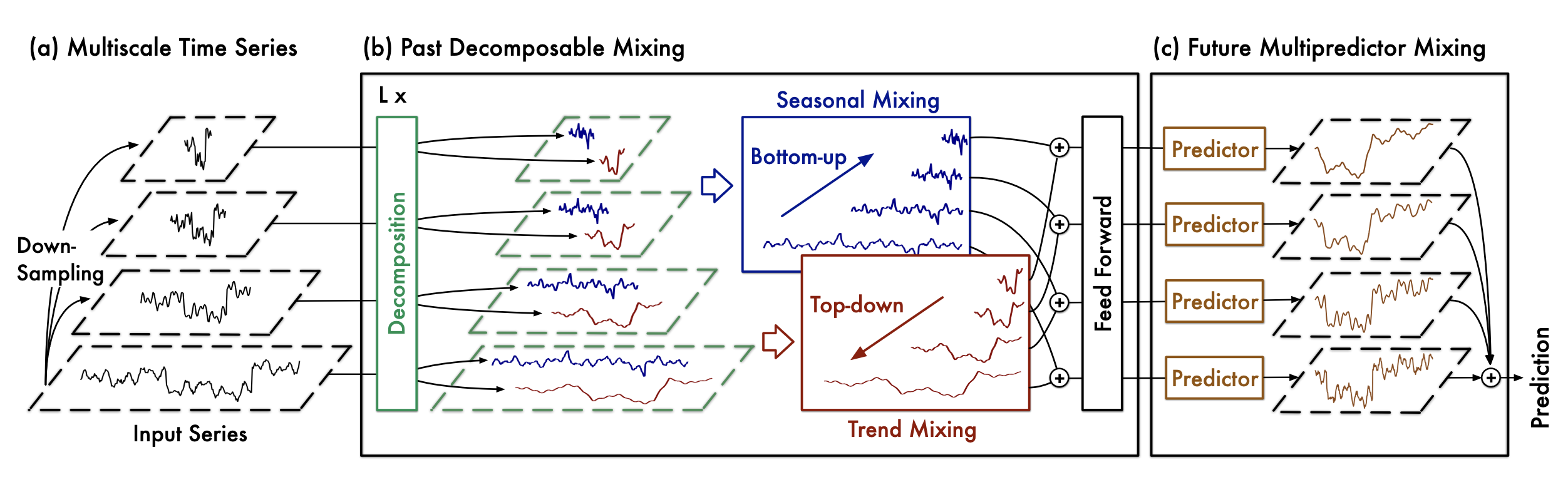
2.2 Mixing
PastDecomposableMixing
PastDecomposableMixing(
    seq_len,
    pred_len,
    down_sampling_window,
    down_sampling_layers,
    d_model,
    dropout,
    channel_independence,
    decomp_method,
    d_ff,
    moving_avg,
    top_k,
)
Module
PastDecomposableMixing
MultiScaleTrendMixing
MultiScaleTrendMixing(seq_len, down_sampling_window, down_sampling_layers)
Module
Top-down mixing trend pattern
MultiScaleSeasonMixing
MultiScaleSeasonMixing(seq_len, down_sampling_window, down_sampling_layers)
Module
Bottom-up mixing season pattern