

LSTM),
uses a multilayer
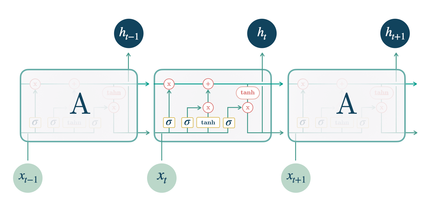
LSTM
encoder and an
MLP
decoder. It builds upon the LSTM-cell that improves the exploding and
vanishing gradients of classic
RNN’s.
This network has been extensively used in sequential prediction tasks
like language modeling, phonetic labeling, and forecasting. The
predictions are obtained by transforming the hidden states into contexts
, that are decoded and adapted into
through MLPs.
where , is the hidden state for time ,
is the input at time and is the
hidden state of the previous layer at , are
static exogenous inputs, historic exogenous,
are future exogenous available at the time
of the prediction.
References
- Jeffrey L. Elman (1990). “Finding Structure in Time”.
- Haşim Sak, Andrew Senior, Françoise Beaufays (2014). “Long Short-Term Memory Based Recurrent Neural Network Architectures for Large Vocabulary Speech Recognition.”
1. LSTM
LSTM
BaseModel
LSTM
LSTM encoder, with MLP decoder.
The network has tanh or relu non-linearities, it is trained using
ADAM stochastic gradient descent. The network accepts static, historic
and future exogenous data.
Parameters:
LSTM.fit
fit method, optimizes the neural network’s weights using the
initialization parameters (learning_rate, windows_batch_size, …)
and the loss function as defined during the initialization.
Within fit we use a PyTorch Lightning Trainer that
inherits the initialization’s self.trainer_kwargs, to customize
its inputs, see PL’s trainer arguments.
The method is designed to be compatible with SKLearn-like classes
and in particular to be compatible with the StatsForecast library.
By default the model is not saving training checkpoints to protect
disk memory, to get them change enable_checkpointing=True in __init__.
Parameters:
Returns:
LSTM.predict
Trainer execution of predict_step.
Parameters:
Returns: