

Fit an LSTM and NHITS modelThis notebook provides an example on how to start using the main functionalities of the NeuralForecast library. The
NeuralForecast
class allows users to easily interact with NeuralForecast.models
PyTorch models. In this example we will forecast AirPassengers data with
a classic LSTM and the recent NHITS models. The full list of
available models is available here.
You can run these experiments using GPU with Google Colab.
1. Installing NeuralForecast
2. Loading AirPassengers Data
Thecore.NeuralForecast class contains shared, fit, predict and
other methods that take as inputs pandas DataFrames with columns
['unique_id', 'ds', 'y'], where unique_id identifies individual time
series from the dataset, ds is the date, and y is the target
variable.
In this example dataset consists of a set of a single series, but you
can easily fit your model to larger datasets in long format.
| unique_id | ds | y | |
|---|---|---|---|
| 0 | 1.0 | 1949-01-31 | 112.0 |
| 1 | 1.0 | 1949-02-28 | 118.0 |
| 2 | 1.0 | 1949-03-31 | 132.0 |
| 3 | 1.0 | 1949-04-30 | 129.0 |
| 4 | 1.0 | 1949-05-31 | 121.0 |
Important DataFrames must include all['unique_id', 'ds', 'y']columns. Make sureycolumn does not have missing or non-numeric values.
3. Model Training
Fit the models
Using theNeuralForecast.fit method you can train a set of models to
your dataset. You can define the forecasting horizon (12 in this
example), and modify the hyperparameters of the model. For example, for
the LSTM we changed the default hidden size for both encoder and
decoders.
Tip The performance of Deep Learning models can be very sensitive to the choice of hyperparameters. Tuning the correct hyperparameters is an important step to obtain the best forecasts. TheAutoversion of these models,AutoLSTMandAutoNHITS, already perform hyperparameter selection automatically.
Predict using the fitted models
Using theNeuralForecast.predict method you can obtain the h
forecasts after the training data Y_df.
NeuralForecast.predict method returns a DataFrame with the
forecasts for each unique_id, ds, and model.
| unique_id | ds | LSTM | NHITS | |
|---|---|---|---|---|
| 0 | 1.0 | 1961-01-31 | 445.602112 | 447.531281 |
| 1 | 1.0 | 1961-02-28 | 431.253510 | 439.081024 |
| 2 | 1.0 | 1961-03-31 | 456.301270 | 481.924194 |
| 3 | 1.0 | 1961-04-30 | 508.149750 | 501.501343 |
| 4 | 1.0 | 1961-05-31 | 524.903870 | 514.664551 |
4. Plot Predictions
Finally, we plot the forecasts of both models against the real values.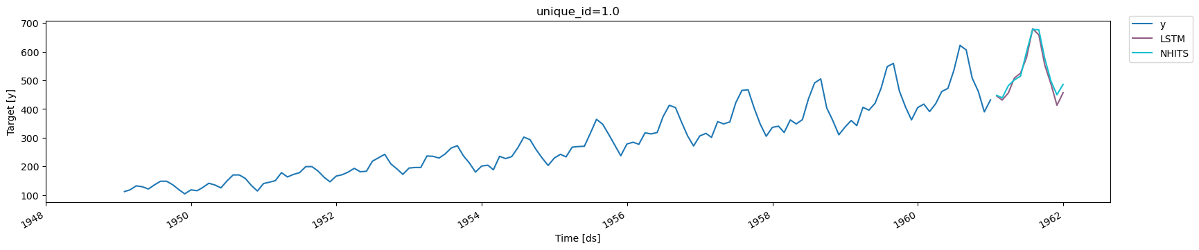
Tip For this guide we are using a simpleLSTMmodel. More recent models, such asTSMixer,TFTandNHITSachieve better accuracy thanLSTMin most settings. The full list of available models is available here.
References
- Boris N. Oreshkin, Dmitri Carpov, Nicolas Chapados, Yoshua Bengio
(2020). “N-BEATS: Neural basis expansion analysis for interpretable
time series forecasting”. International Conference on Learning
Representations.
- Cristian Challu, Kin G. Olivares, Boris N. Oreshkin, Federico Garza, Max Mergenthaler-Canseco, Artur Dubrawski (2021). NHITS: Neural Hierarchical Interpolation for Time Series Forecasting. Accepted at AAAI 2023.