NBEATS

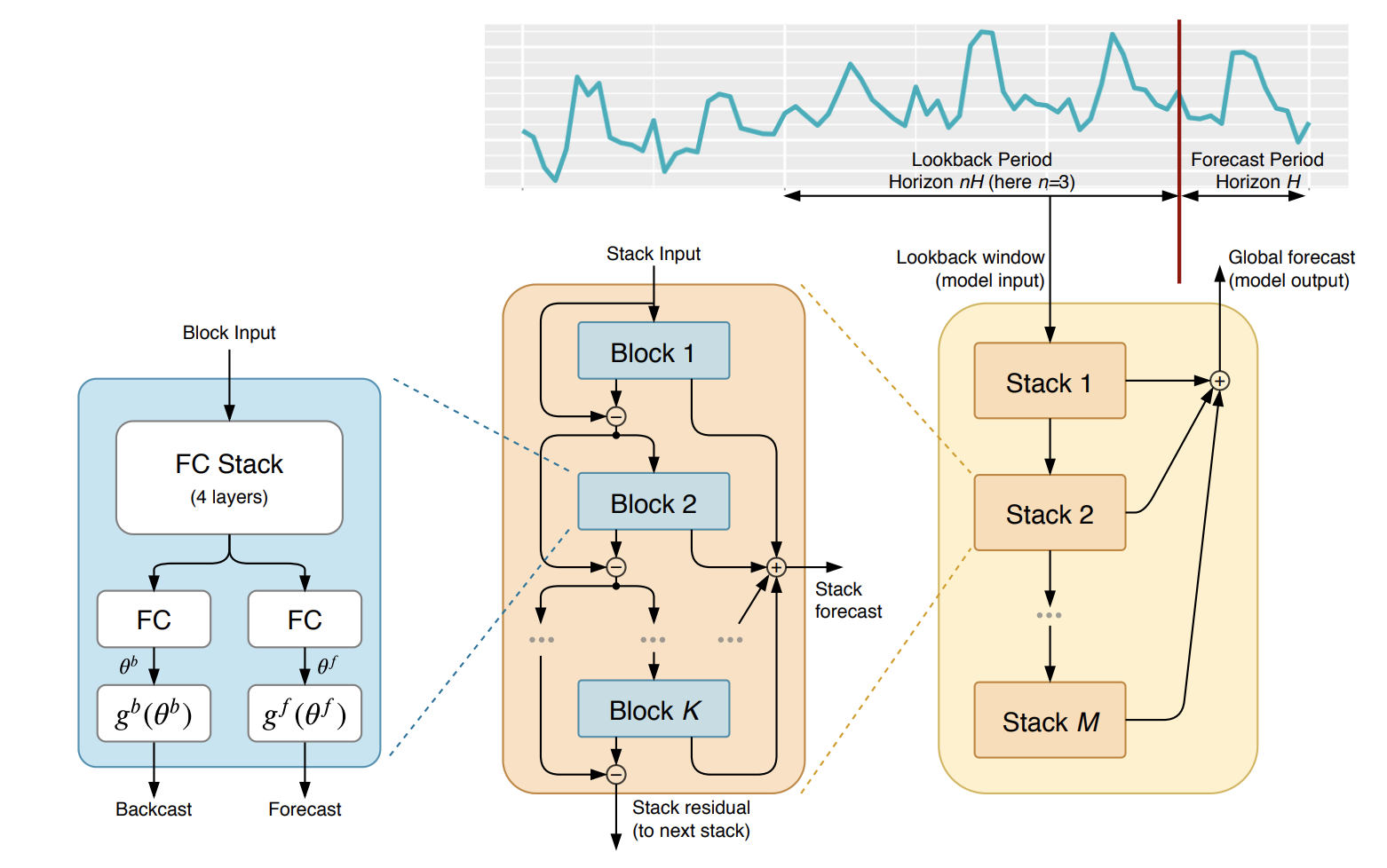
The Neural Basis Expansion Analysis (NBEATS) is an MLP-based deep neural architecture with backward and forward residual links. The network has two variants: (1) in its interpretable configuration, NBEATS sequentially projects the signal into polynomials and harmonic basis to learn trend and seasonality components; (2) in its generic configuration, it substitutes the polynomial and harmonic basis for identity basis and larger network’s depth. The Neural Basis Expansion Analysis with Exogenous (NBEATSx), incorporates projections to exogenous temporal variables available at the time of the prediction.

This method proved state-of-the-art performance on the M3, M4, and Tourism Competition datasets, improving accuracy by 3% over the ESRNN M4 competition winner.

References
-Boris N. Oreshkin, Dmitri Carpov, Nicolas Chapados, Yoshua Bengio (2019). “N-BEATS: Neural basis expansion analysis for interpretable time series forecasting”.

​

NBEATS

 NBEATS (h, input_size, n_harmonics:int=2, n_polynomials:int=2,
         stack_types:list=['identity', 'trend', 'seasonality'],
         n_blocks:list=[1, 1, 1], mlp_units:list=[[512, 512], [512, 512],
         [512, 512]], dropout_prob_theta:float=0.0, activation:str='ReLU',
         shared_weights:bool=False, loss=MAE(), valid_loss=None,
         max_steps:int=1000, learning_rate:float=0.001,
         num_lr_decays:int=3, early_stop_patience_steps:int=-1,
         val_check_steps:int=100, batch_size:int=32,
         valid_batch_size:Optional[int]=None, windows_batch_size:int=1024,
         inference_windows_batch_size:int=-1, start_padding_enabled=False,
         step_size:int=1, scaler_type:str='identity', random_seed:int=1,
         num_workers_loader:int=0, drop_last_loader:bool=False,
         optimizer=None, optimizer_kwargs=None, **trainer_kwargs)

*NBEATS

The Neural Basis Expansion Analysis for Time Series (NBEATS), is a simple and yet effective architecture, it is built with a deep stack of MLPs with the doubly residual connections. It has a generic and interpretable architecture depending on the blocks it uses. Its interpretable architecture is recommended for scarce data settings, as it regularizes its predictions through projections unto harmonic and trend basis well-suited for most forecasting tasks.

Parameters:
h: int, forecast horizon.
input_size: int, considered autorregresive inputs (lags), y=[1,2,3,4] input_size=2 -> lags=[1,2].
n_harmonics: int, Number of harmonic terms for seasonality stack type. Note that len(n_harmonics) = len(stack_types). Note that it will only be used if a seasonality stack is used.
n_polynomials: int, polynomial degree for trend stack. Note that len(n_polynomials) = len(stack_types). Note that it will only be used if a trend stack is used.
stack_types: List[str], List of stack types. Subset from [‘seasonality’, ‘trend’, ‘identity’].
n_blocks: List[int], Number of blocks for each stack. Note that len(n_blocks) = len(stack_types).
mlp_units: List[List[int]], Structure of hidden layers for each stack type. Each internal list should contain the number of units of each hidden layer. Note that len(n_hidden) = len(stack_types).
dropout_prob_theta: float, Float between (0, 1). Dropout for N-BEATS basis.
shared_weights: bool, If True, all blocks within each stack will share parameters.
activation: str, activation from [‘ReLU’, ‘Softplus’, ‘Tanh’, ‘SELU’, ‘LeakyReLU’, ‘PReLU’, ‘Sigmoid’].
loss: PyTorch module, instantiated train loss class from losses collection.
valid_loss: PyTorch module=loss, instantiated valid loss class from losses collection.
max_steps: int=1000, maximum number of training steps.
learning_rate: float=1e-3, Learning rate between (0, 1).
num_lr_decays: int=3, Number of learning rate decays, evenly distributed across max_steps.
early_stop_patience_steps: int=-1, Number of validation iterations before early stopping.
val_check_steps: int=100, Number of training steps between every validation loss check.
batch_size: int=32, number of different series in each batch.
valid_batch_size: int=None, number of different series in each validation and test batch, if None uses batch_size.
windows_batch_size: int=1024, number of windows to sample in each training batch, default uses all.
inference_windows_batch_size: int=-1, number of windows to sample in each inference batch, -1 uses all.
start_padding_enabled: bool=False, if True, the model will pad the time series with zeros at the beginning, by input size.
step_size: int=1, step size between each window of temporal data.
scaler_type: str=‘identity’, type of scaler for temporal inputs normalization see temporal scalers.
random_seed: int, random_seed for pytorch initializer and numpy generators.
num_workers_loader: int=os.cpu_count(), workers to be used by TimeSeriesDataLoader.
drop_last_loader: bool=False, if True TimeSeriesDataLoader drops last non-full batch.
alias: str, optional, Custom name of the model.
optimizer: Subclass of ‘torch.optim.Optimizer’, optional, user specified optimizer instead of the default choice (Adam).
optimizer_kwargs: dict, optional, list of parameters used by the user specified optimizer.
**trainer_kwargs: int, keyword trainer arguments inherited from PyTorch Lighning’s trainer.

References:
-Boris N. Oreshkin, Dmitri Carpov, Nicolas Chapados, Yoshua Bengio (2019). “N-BEATS: Neural basis expansion analysis for interpretable time series forecasting”.*

​

NBEATS.fit

 NBEATS.fit (dataset, val_size=0, test_size=0, random_seed=None,
             distributed_config=None)

*Fit.

The fit method, optimizes the neural network’s weights using the initialization parameters (learning_rate, windows_batch_size, …) and the loss function as defined during the initialization. Within fit we use a PyTorch Lightning Trainer that inherits the initialization’s self.trainer_kwargs, to customize its inputs, see PL’s trainer arguments.

The method is designed to be compatible with SKLearn-like classes and in particular to be compatible with the StatsForecast library.

By default the model is not saving training checkpoints to protect disk memory, to get them change enable_checkpointing=True in __init__.

Parameters:
dataset: NeuralForecast’s TimeSeriesDataset, see documentation.
val_size: int, validation size for temporal cross-validation.
random_seed: int=None, random_seed for pytorch initializer and numpy generators, overwrites model.__init__’s.
test_size: int, test size for temporal cross-validation.
*

​

NBEATS.predict

 NBEATS.predict (dataset, test_size=None, step_size=1, random_seed=None,
                 **data_module_kwargs)

*Predict.

Neural network prediction with PL’s Trainer execution of predict_step.

Parameters:
dataset: NeuralForecast’s TimeSeriesDataset, see documentation.
test_size: int=None, test size for temporal cross-validation.
step_size: int=1, Step size between each window.
random_seed: int=None, random_seed for pytorch initializer and numpy generators, overwrites model.__init__’s.
**data_module_kwargs: PL’s TimeSeriesDataModule args, see documentation.*

​

Usage Example

import numpy as np
import pandas as pd
import pytorch_lightning as pl
import matplotlib.pyplot as plt

from neuralforecast import NeuralForecast
from neuralforecast.models import NBEATS
from neuralforecast.losses.pytorch import MQLoss, DistributionLoss
from neuralforecast.tsdataset import TimeSeriesDataset
from neuralforecast.utils import AirPassengers, AirPassengersPanel, AirPassengersStatic

Y_train_df = AirPassengersPanel[AirPassengersPanel.ds<AirPassengersPanel['ds'].values[-12]] # 132 train
Y_test_df = AirPassengersPanel[AirPassengersPanel.ds>=AirPassengersPanel['ds'].values[-12]].reset_index(drop=True) # 12 test

model = NBEATS(h=12, input_size=24,
               loss=DistributionLoss(distribution='Poisson', level=[80, 90]),
               stack_types = ['identity', 'trend', 'seasonality'],
               max_steps=100,
               val_check_steps=10,
               early_stop_patience_steps=2)

fcst = NeuralForecast(
    models=[model],
    freq='M'
)
fcst.fit(df=Y_train_df, static_df=AirPassengersStatic, val_size=12)
forecasts = fcst.predict(futr_df=Y_test_df)

# Plot quantile predictions
Y_hat_df = forecasts.reset_index(drop=False).drop(columns=['unique_id','ds'])
plot_df = pd.concat([Y_test_df, Y_hat_df], axis=1)
plot_df = pd.concat([Y_train_df, plot_df])

plot_df = plot_df[plot_df.unique_id=='Airline1'].drop('unique_id', axis=1)
plt.plot(plot_df['ds'], plot_df['y'], c='black', label='True')
plt.plot(plot_df['ds'], plot_df['NBEATS-median'], c='blue', label='median')
plt.fill_between(x=plot_df['ds'][-12:], 
                 y1=plot_df['NBEATS-lo-90'][-12:].values, 
                 y2=plot_df['NBEATS-hi-90'][-12:].values,
                 alpha=0.4, label='level 90')
plt.grid()
plt.legend()
plt.plot()