NHITS

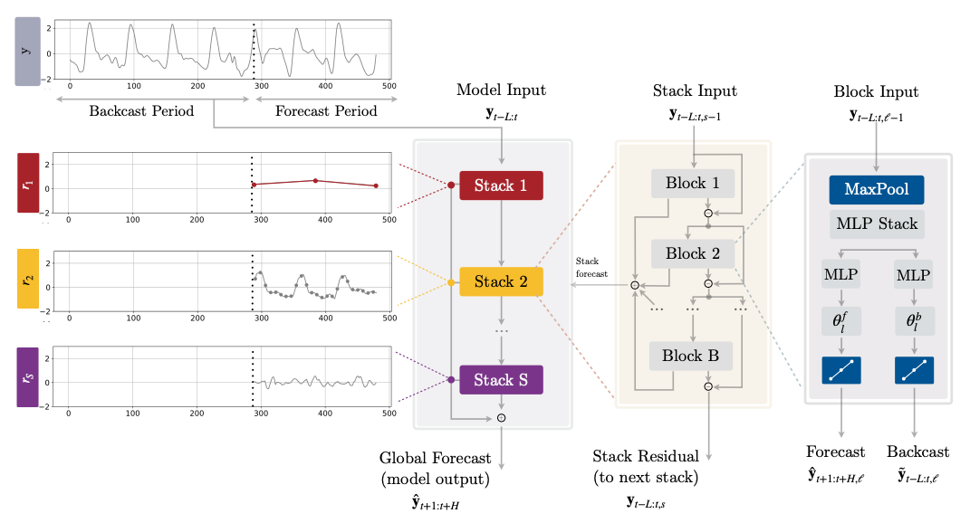
Long-horizon forecasting is challenging because of the volatility of the predictions and the computational complexity. To solve this problem we created the Neural Hierarchical Interpolation for Time Series (NHITS). NHITS builds upon NBEATS and specializes its partial outputs in the different frequencies of the time series through hierarchical interpolation and multi-rate input processing. On the long-horizon forecasting task NHITS improved accuracy by 25% on AAAI’s best paper award the Informer, while being 50x faster.

The model is composed of several MLPs with ReLU non-linearities. Blocks are connected via doubly residual stacking principle with the backcast $\mathbf{\tilde{y}}_{t-L:t,l}$ and forecast $\mathbf{\hat{y}}_{t+1:t+H,l}$ outputs of the l-th block. Multi-rate input pooling, hierarchical interpolation and backcast residual connections together induce the specialization of the additive predictions in different signal bands, reducing memory footprint and computational time, thus improving the architecture parsimony and accuracy.

References
-Boris N. Oreshkin, Dmitri Carpov, Nicolas Chapados, Yoshua Bengio (2019). “N-BEATS: Neural basis expansion analysis for interpretable time series forecasting”.
-Cristian Challu, Kin G. Olivares, Boris N. Oreshkin, Federico Garza, Max Mergenthaler-Canseco, Artur Dubrawski (2023). “NHITS: Neural Hierarchical Interpolation for Time Series Forecasting”. Accepted at the Thirty-Seventh AAAI Conference on Artificial Intelligence.
-Zhou, H.; Zhang, S.; Peng, J.; Zhang, S.; Li, J.; Xiong, H.; and Zhang, W. (2020). “Informer: Beyond Efficient Transformer for Long Sequence Time-Series Forecasting”. Association for the Advancement of Artificial Intelligence Conference 2021 (AAAI 2021).

source

 NHITS (h, input_size, futr_exog_list=None, hist_exog_list=None,
        stat_exog_list=None, exclude_insample_y=False,
        stack_types:list=['identity', 'identity', 'identity'],
        n_blocks:list=[1, 1, 1], mlp_units:list=[[512, 512], [512, 512],
        [512, 512]], n_pool_kernel_size:list=[2, 2, 1],
        n_freq_downsample:list=[4, 2, 1], pooling_mode:str='MaxPool1d',
        interpolation_mode:str='linear', dropout_prob_theta=0.0,
        activation='ReLU', loss=MAE(), valid_loss=None,
        max_steps:int=1000, learning_rate:float=0.001,
        num_lr_decays:int=3, early_stop_patience_steps:int=-1,
        val_check_steps:int=100, batch_size:int=32,
        valid_batch_size:Optional[int]=None, windows_batch_size:int=1024,
        inference_windows_batch_size:int=-1, start_padding_enabled=False,
        step_size:int=1, scaler_type:str='identity', random_seed:int=1,
        num_workers_loader=0, drop_last_loader=False, optimizer=None,
        optimizer_kwargs=None, **trainer_kwargs)

*NHITS

The Neural Hierarchical Interpolation for Time Series (NHITS), is an MLP-based deep neural architecture with backward and forward residual links. NHITS tackles volatility and memory complexity challenges, by locally specializing its sequential predictions into the signals frequencies with hierarchical interpolation and pooling.

Parameters:
h: int, Forecast horizon.
input_size: int, autorregresive inputs size, y=[1,2,3,4] input_size=2 -> y_[t-2:t]=[1,2].
stat_exog_list: str list, static exogenous columns.
hist_exog_list: str list, historic exogenous columns.
futr_exog_list: str list, future exogenous columns.
exclude_insample_y: bool=False, the model skips the autoregressive features y[t-input_size:t] if True.
activation: str, activation from [‘ReLU’, ‘Softplus’, ‘Tanh’, ‘SELU’, ‘LeakyReLU’, ‘PReLU’, ‘Sigmoid’].
stack_types: List[str], stacks list in the form N * [‘identity’], to be deprecated in favor of n_stacks. Note that len(stack_types)=len(n_freq_downsample)=len(n_pool_kernel_size).
n_blocks: List[int], Number of blocks for each stack. Note that len(n_blocks) = len(stack_types).
mlp_units: List[List[int]], Structure of hidden layers for each stack type. Each internal list should contain the number of units of each hidden layer. Note that len(n_hidden) = len(stack_types).
n_freq_downsample: List[int], list with the stack’s coefficients (inverse expressivity ratios). Note that len(stack_types)=len(n_freq_downsample)=len(n_pool_kernel_size).
interpolation_mode: str=‘linear’, interpolation basis from [‘linear’, ‘nearest’, ‘cubic’].
n_pool_kernel_size: List[int], list with the size of the windows to take a max/avg over. Note that len(stack_types)=len(n_freq_downsample)=len(n_pool_kernel_size).
pooling_mode: str, input pooling module from [‘MaxPool1d’, ‘AvgPool1d’].
dropout_prob_theta: float, Float between (0, 1). Dropout for NHITS basis.
loss: PyTorch module, instantiated train loss class from losses collection.
valid_loss: PyTorch module=loss, instantiated valid loss class from losses collection.
max_steps: int=1000, maximum number of training steps.
learning_rate: float=1e-3, Learning rate between (0, 1).
num_lr_decays: int=-1, Number of learning rate decays, evenly distributed across max_steps.
early_stop_patience_steps: int=-1, Number of validation iterations before early stopping.
val_check_steps: int=100, Number of training steps between every validation loss check.
batch_size: int=32, number of different series in each batch.
valid_batch_size: int=None, number of different series in each validation and test batch, if None uses batch_size.
windows_batch_size: int=1024, number of windows to sample in each training batch, default uses all.
inference_windows_batch_size: int=-1, number of windows to sample in each inference batch, -1 uses all.
start_padding_enabled: bool=False, if True, the model will pad the time series with zeros at the beginning, by input size.
step_size: int=1, step size between each window of temporal data.
scaler_type: str=‘identity’, type of scaler for temporal inputs normalization see temporal scalers.
random_seed: int, random_seed for pytorch initializer and numpy generators.
num_workers_loader: int=os.cpu_count(), workers to be used by TimeSeriesDataLoader.
drop_last_loader: bool=False, if True TimeSeriesDataLoader drops last non-full batch.
alias: str, optional, Custom name of the model.
optimizer: Subclass of ‘torch.optim.Optimizer’, optional, user specified optimizer instead of the default choice (Adam).
optimizer_kwargs: dict, optional, list of parameters used by the user specified optimizer.
**trainer_kwargs: int, keyword trainer arguments inherited from PyTorch Lighning’s trainer.

References:
-Cristian Challu, Kin G. Olivares, Boris N. Oreshkin, Federico Garza, Max Mergenthaler-Canseco, Artur Dubrawski (2023). “NHITS: Neural Hierarchical Interpolation for Time Series Forecasting”. Accepted at the Thirty-Seventh AAAI Conference on Artificial Intelligence.*

NHITS.fit

 NHITS.fit (dataset, val_size=0, test_size=0, random_seed=None,
            distributed_config=None)

*Fit.

The fit method, optimizes the neural network’s weights using the initialization parameters (learning_rate, windows_batch_size, …) and the loss function as defined during the initialization. Within fit we use a PyTorch Lightning Trainer that inherits the initialization’s self.trainer_kwargs, to customize its inputs, see PL’s trainer arguments.

The method is designed to be compatible with SKLearn-like classes and in particular to be compatible with the StatsForecast library.

By default the model is not saving training checkpoints to protect disk memory, to get them change enable_checkpointing=True in __init__.

Parameters:
dataset: NeuralForecast’s TimeSeriesDataset, see documentation.
val_size: int, validation size for temporal cross-validation.
random_seed: int=None, random_seed for pytorch initializer and numpy generators, overwrites model.__init__’s.
test_size: int, test size for temporal cross-validation.
*

NHITS.predict

 NHITS.predict (dataset, test_size=None, step_size=1, random_seed=None,
                **data_module_kwargs)

*Predict.

Neural network prediction with PL’s Trainer execution of predict_step.

Parameters:
dataset: NeuralForecast’s TimeSeriesDataset, see documentation.
test_size: int=None, test size for temporal cross-validation.
step_size: int=1, Step size between each window.
random_seed: int=None, random_seed for pytorch initializer and numpy generators, overwrites model.__init__’s.
**data_module_kwargs: PL’s TimeSeriesDataModule args, see documentation.*

Usage Example

import numpy as np
import pandas as pd
import pytorch_lightning as pl
import matplotlib.pyplot as plt

from neuralforecast import NeuralForecast
from neuralforecast.models import NHITS
from neuralforecast.losses.pytorch import MQLoss, DistributionLoss, PMM, GMM, NBMM
from neuralforecast.tsdataset import TimeSeriesDataset
from neuralforecast.utils import AirPassengers, AirPassengersPanel, AirPassengersStatic


Y_train_df = AirPassengersPanel[AirPassengersPanel.ds<AirPassengersPanel['ds'].values[-12]].reset_index(drop=True) # 132 train
Y_test_df = AirPassengersPanel[AirPassengersPanel.ds>=AirPassengersPanel['ds'].values[-12]].reset_index(drop=True) # 12 test

model = NHITS(h=12,
              input_size=24,
              loss=DistributionLoss(distribution='StudentT', level=[80, 90], return_params=True),
              #loss=DistributionLoss(distribution='Normal', level=[80, 90], return_params=True),
              #loss=DistributionLoss(distribution='Poisson', level=[80, 90], return_params=True),
              #loss=DistributionLoss(distribution='Tweedie', level=[80, 90], rho=1.5),
              #loss=DistributionLoss(distribution='NegativeBinomial', level=[80, 90], return_params=True),
              #loss=NBMM(n_components=2, level=[80,90]),
              #loss=GMM(n_components=2, level=[80,90]),
              #loss=PMM(n_components=1, level=[80,90]),
              stat_exog_list=['airline1'],
              futr_exog_list=['trend'],
              n_freq_downsample=[2, 1, 1],
              scaler_type='robust',
              max_steps=200,
              early_stop_patience_steps=2,
              inference_windows_batch_size=1,
              val_check_steps=10,
              learning_rate=1e-3)

fcst = NeuralForecast(models=[model], freq='M')
fcst.fit(df=Y_train_df, static_df=AirPassengersStatic, val_size=12)
forecasts = fcst.predict(futr_df=Y_test_df)

# Plot quantile predictions
Y_hat_df = forecasts.reset_index(drop=False).drop(columns=['unique_id','ds'])
plot_df = pd.concat([Y_test_df, Y_hat_df], axis=1)
plot_df = pd.concat([Y_train_df, plot_df])

plot_df = plot_df[plot_df.unique_id=='Airline1'].drop('unique_id', axis=1)
plt.plot(plot_df['ds'], plot_df['y'], c='black', label='True')
plt.plot(plot_df['ds'], plot_df['NHITS-median'], c='blue', label='median')
plt.fill_between(x=plot_df['ds'][-12:], 
                 y1=plot_df['NHITS-lo-90'][-12:].values, 
                 y2=plot_df['NHITS-hi-90'][-12:].values,
                 alpha=0.4, label='level 90')
plt.legend()
plt.grid()
plt.plot()

import numpy as np
import pandas as pd
import pytorch_lightning as pl
import matplotlib.pyplot as plt

from neuralforecast import NeuralForecast
from neuralforecast.models import NHITS
from neuralforecast.losses.pytorch import DistributionLoss, HuberLoss, MAE
from neuralforecast.tsdataset import TimeSeriesDataset
from neuralforecast.utils import AirPassengers, AirPassengersPanel, AirPassengersStatic

#AirPassengersPanel['y'] = 1 * (AirPassengersPanel['trend'] % 12) < 2
Y_train_df = AirPassengersPanel[AirPassengersPanel.ds<AirPassengersPanel['ds'].values[-12]].reset_index(drop=True) # 132 train
Y_test_df = AirPassengersPanel[AirPassengersPanel.ds>=AirPassengersPanel['ds'].values[-12]].reset_index(drop=True) # 12 test

model = NHITS(h=12,
              input_size=24,
              #loss=DistributionLoss(distribution='StudentT', level=[80, 90], return_params=True),
              loss=HuberLoss(delta=0.5),
              valid_loss=MAE(),
              stat_exog_list=['airline1'],
              scaler_type='robust',
              max_steps=200,
              early_stop_patience_steps=2,
              val_check_steps=10,
              learning_rate=1e-3)

fcst = NeuralForecast(models=[model], freq='M')
fcst.fit(df=Y_train_df, static_df=AirPassengersStatic, val_size=12)
forecasts = fcst.predict(futr_df=Y_test_df)

# Plot quantile predictions
Y_hat_df = forecasts.reset_index(drop=False).drop(columns=['unique_id','ds'])
plot_df = pd.concat([Y_test_df, Y_hat_df], axis=1)
plot_df = pd.concat([Y_train_df, plot_df])

plot_df = plot_df[plot_df.unique_id=='Airline1'].drop('unique_id', axis=1)
plt.plot(plot_df['ds'], plot_df['y'], c='black', label='True')
plt.plot(plot_df['ds'], plot_df['NHITS'], c='blue', label='median')
# plt.plot(plot_df['ds'], plot_df['NHITS-median'], c='blue', label='median')
# plt.fill_between(x=plot_df['ds'][-12:], 
#                  y1=plot_df['NHITS-lo-90'][-12:].values, 
#                  y2=plot_df['NHITS-hi-90'][-12:].values,
#                  alpha=0.4, label='level 90')
plt.legend()
plt.grid()
plt.plot()

Getting Started

Tutorials

API Reference

NHITS

NHITS

NHITS.fit

NHITS.predict

Usage Example

Getting Started

Tutorials

API Reference

​NHITS

​NHITS.fit

​NHITS.predict

​Usage Example

NHITS

NHITS.fit

NHITS.predict

Usage Example