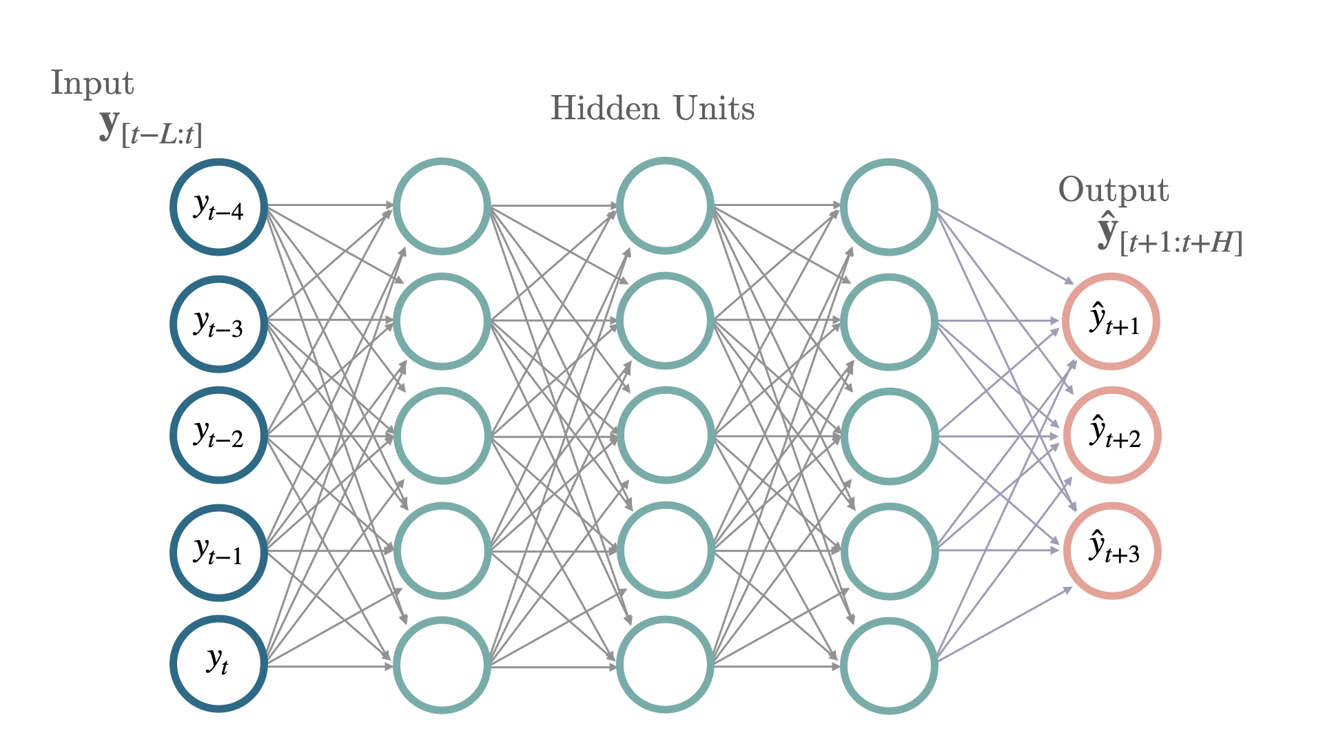
One of the simplest neural architectures are Multi Layer Perceptrons (MLP) composed of stacked Fully Connected Neural Networks trained with backpropagation. Each node in the architecture is capable of modeling non-linear relationships granted by their activation functions. Novel activations like Rectified Linear Units (ReLU) have greatly improved the ability to fit deeper networks overcoming gradient vanishing problems that were associated with Sigmoid and TanH activations. For the forecasting task the last layer is changed to follow a auto-regression problem. This version is multivariate, indicating that it will predict all time series of the forecasting problem jointly. References -Rosenblatt, F. (1958). “The perceptron: A probabilistic model for information storage and organization in the brain.” -Fukushima, K. (1975). “Cognitron: A self-organizing multilayered neural network.” -Vinod Nair, Geoffrey E. Hinton (2010). “Rectified Linear Units Improve Restricted Boltzmann Machines” Figure 1. Three layer MLP with autorregresive inputs. Figure 1. Three layer MLP with autorregresive inputs.

MLPMultivariate

MLPMultivariate

MLPMultivariate(
    h,
    input_size,
    n_series,
    stat_exog_list=None,
    hist_exog_list=None,
    futr_exog_list=None,
    exclude_insample_y=False,
    num_layers=2,
    hidden_size=1024,
    loss=MAE(),
    valid_loss=None,
    max_steps=1000,
    learning_rate=0.001,
    num_lr_decays=-1,
    early_stop_patience_steps=-1,
    val_check_steps=100,
    batch_size=32,
    valid_batch_size=None,
    windows_batch_size=32,
    inference_windows_batch_size=32,
    start_padding_enabled=False,
    training_data_availability_threshold=0.0,
    step_size=1,
    scaler_type="identity",
    random_seed=1,
    drop_last_loader=False,
    alias=None,
    optimizer=None,
    optimizer_kwargs=None,
    lr_scheduler=None,
    lr_scheduler_kwargs=None,
    dataloader_kwargs=None,
    **trainer_kwargs
)
Bases: BaseModel MLPMultivariate Simple Multi Layer Perceptron architecture (MLP) for multivariate forecasting. This deep neural network has constant units through its layers, each with ReLU non-linearities, it is trained using ADAM stochastic gradient descent. The network accepts static, historic and future exogenous data, flattens the inputs and learns fully connected relationships against the target variables. Parameters:
NameTypeDescriptionDefault
hintforecast horizon.required
input_sizeintconsidered autorregresive inputs (lags), y=[1,2,3,4] input_size=2 -> lags=[1,2].required
n_seriesintnumber of time-series.required
stat_exog_liststr liststatic exogenous columns.None
hist_exog_liststr listhistoric exogenous columns.None
futr_exog_liststr listfuture exogenous columns.None
num_layersintnumber of layers for the MLP.2
hidden_sizeintnumber of units for each layer of the MLP.1024
lossPyTorch moduleinstantiated train loss class from losses collection.MAE()
valid_lossPyTorch moduleinstantiated valid loss class from losses collection.None
max_stepsintmaximum number of training steps.1000
learning_ratefloatLearning rate between (0, 1).0.001
num_lr_decaysintNumber of learning rate decays, evenly distributed across max_steps.-1
early_stop_patience_stepsintNumber of validation iterations before early stopping.-1
val_check_stepsintNumber of training steps between every validation loss check.100
batch_sizeintnumber of different series in each batch.32
valid_batch_sizeintnumber of different series in each validation and test batch, if None uses batch_size.None
windows_batch_sizeintnumber of windows to sample in each training batch, default uses all.32
inference_windows_batch_sizeintnumber of windows to sample in each inference batch, -1 uses all.32
start_padding_enabledboolif True, the model will pad the time series with zeros at the beginning, by input size.False
training_data_availability_thresholdUnion[float, List[float]]minimum fraction of valid data points required for training windows. Single float applies to both insample and outsample; list of two floats specifies [insample_fraction, outsample_fraction]. Default 0.0 allows windows with only 1 valid data point (current behavior).0.0
step_sizeintstep size between each window of temporal data.1
scaler_typestrtype of scaler for temporal inputs normalization see temporal scalers.‘identity’
random_seedintrandom_seed for pytorch initializer and numpy generators.1
drop_last_loaderboolif True TimeSeriesDataLoader drops last non-full batch.False
aliasstroptional, Custom name of the model.None
optimizerSubclass of ‘torch.optim.Optimizer’optional, user specified optimizer instead of the default choice (Adam).None
optimizer_kwargsdictoptional, list of parameters used by the user specified optimizer.None
lr_schedulerSubclass of ‘torch.optim.lr_scheduler.LRScheduler’optional, user specified lr_scheduler instead of the default choice (StepLR).None
lr_scheduler_kwargsdictoptional, list of parameters used by the user specified lr_scheduler.None
dataloader_kwargsdictoptional, list of parameters passed into the PyTorch Lightning dataloader by the TimeSeriesDataLoader.None
**trainer_kwargsintkeyword trainer arguments inherited from PyTorch Lighning’s trainer.

MLPMultivariate.fit

fit(
    dataset, val_size=0, test_size=0, random_seed=None, distributed_config=None
)
Fit. The fit method, optimizes the neural network’s weights using the initialization parameters (learning_rate, windows_batch_size, …) and the loss function as defined during the initialization. Within fit we use a PyTorch Lightning Trainer that inherits the initialization’s self.trainer_kwargs, to customize its inputs, see PL’s trainer arguments. The method is designed to be compatible with SKLearn-like classes and in particular to be compatible with the StatsForecast library. By default the model is not saving training checkpoints to protect disk memory, to get them change enable_checkpointing=True in __init__. Parameters:
NameTypeDescriptionDefault
datasetTimeSeriesDatasetNeuralForecast’s TimeSeriesDataset, see documentation.required
val_sizeintValidation size for temporal cross-validation.0
random_seedintRandom seed for pytorch initializer and numpy generators, overwrites model.init’s.None
test_sizeintTest size for temporal cross-validation.0
Returns:
TypeDescription
None

MLPMultivariate.predict

predict(
    dataset,
    test_size=None,
    step_size=1,
    random_seed=None,
    quantiles=None,
    h=None,
    explainer_config=None,
    **data_module_kwargs
)
Predict. Neural network prediction with PL’s Trainer execution of predict_step. Parameters:
NameTypeDescriptionDefault
datasetTimeSeriesDatasetNeuralForecast’s TimeSeriesDataset, see documentation.required
test_sizeintTest size for temporal cross-validation.None
step_sizeintStep size between each window.1
random_seedintRandom seed for pytorch initializer and numpy generators, overwrites model.init’s.None
quantileslistTarget quantiles to predict.None
hintPrediction horizon, if None, uses the model’s fitted horizon. Defaults to None.None
explainer_configdictconfiguration for explanations.None
**data_module_kwargsdictPL’s TimeSeriesDataModule args, see documentation.
Returns:
TypeDescription
None

Usage Example

import pandas as pd
import matplotlib.pyplot as plt

from neuralforecast import NeuralForecast
from neuralforecast.models import MLPMultivariate
from neuralforecast.losses.pytorch import MAE
from neuralforecast.utils import AirPassengersPanel, AirPassengersStatic

Y_train_df = AirPassengersPanel[AirPassengersPanel.ds<AirPassengersPanel['ds'].values[-12]] # 132 train
Y_test_df = AirPassengersPanel[AirPassengersPanel.ds>=AirPassengersPanel['ds'].values[-12]].reset_index(drop=True) # 12 test

model = MLPMultivariate(h=12, 
            input_size=24,
            n_series=2,
            stat_exog_list=['airline1'],
            futr_exog_list=['trend'],            
            loss = MAE(),
            scaler_type='robust',
            learning_rate=1e-3,
            stat_exog_list=['airline1'],
            max_steps=200,
            val_check_steps=10,
            early_stop_patience_steps=2)

fcst = NeuralForecast(
    models=[model],
    freq='ME'
)
fcst.fit(df=Y_train_df, static_df=AirPassengersStatic, val_size=12)
forecasts = fcst.predict(futr_df=Y_test_df)

# Plot predictions
Y_hat_df = forecasts.reset_index(drop=False).drop(columns=['unique_id','ds'])
plot_df = pd.concat([Y_test_df, Y_hat_df], axis=1)
plot_df = pd.concat([Y_train_df, plot_df])

plot_df = plot_df[plot_df.unique_id=='Airline1'].drop('unique_id', axis=1)
plt.plot(plot_df['ds'], plot_df['y'], c='black', label='True')
plt.plot(plot_df['ds'], plot_df['MLPMultivariate'], c='blue', label='median')
plt.grid()
plt.legend()
plt.plot()