

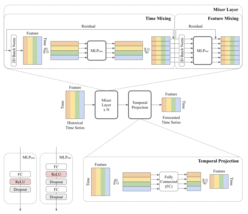
TSMixer) is a MLP-based multivariate time-series
forecasting model. TSMixer jointly learns temporal and cross-sectional
representations of the time-series by repeatedly combining time- and feature
information using stacked mixing layers. A mixing layer consists of a
sequential time- and feature Multi Layer Perceptron (MLP). Note: this model
cannot handle exogenous inputs. If you want to use additional exogenous
inputs, use TSMixerx.
1. TSMixer
TSMixer
BaseModel
TSMixer
Time-Series Mixer (TSMixer) is a MLP-based multivariate time-series forecasting model. TSMixer jointly learns temporal and cross-sectional representations of the time-series by repeatedly combining time- and feature information using stacked mixing layers. A mixing layer consists of a sequential time- and feature Multi Layer Perceptron (MLP).
Parameters:
| Name | Type | Description | Default |
|---|---|---|---|
h | int | forecast horizon. | required |
input_size | int | considered autorregresive inputs (lags), y=[1,2,3,4] input_size=2 -> lags=[1,2]. | required |
n_series | int | number of time-series. | required |
futr_exog_list | str list | future exogenous columns. | None |
hist_exog_list | str list | historic exogenous columns. | None |
stat_exog_list | str list | static exogenous columns. | None |
exclude_insample_y | bool | if True excludes the target variable from the input features. | False |
n_block | int | number of mixing layers in the model. | 2 |
ff_dim | int | number of units for the second feed-forward layer in the feature MLP. | 64 |
dropout | float | dropout rate between (0, 1) . | 0.9 |
revin | bool | if True uses Reverse Instance Normalization to process inputs and outputs. | True |
loss | PyTorch module | instantiated train loss class from losses collection. | MAE() |
valid_loss | PyTorch module | instantiated valid loss class from losses collection. | None |
max_steps | int | maximum number of training steps. | 1000 |
learning_rate | float | Learning rate between (0, 1). | 0.001 |
num_lr_decays | int | Number of learning rate decays, evenly distributed across max_steps. | -1 |
early_stop_patience_steps | int | Number of validation iterations before early stopping. | -1 |
val_monitor | str | metric to monitor for early stopping. Valid options: “ptl/val_loss”, “valid_loss”, “train_loss”. Default: “ptl/val_loss”. | ‘ptl/val_loss’ |
val_check_steps | int | Number of training steps between every validation loss check. | 100 |
batch_size | int | number of different series in each batch. | 32 |
valid_batch_size | int | number of different series in each validation and test batch, if None uses batch_size. | None |
windows_batch_size | int | number of windows to sample in each training batch, default uses all. | 32 |
inference_windows_batch_size | int | number of windows to sample in each inference batch, -1 uses all. | 32 |
start_padding_enabled | bool | if True, the model will pad the time series with zeros at the beginning, by input size. | False |
training_data_availability_threshold | Union[float, List[float]] | minimum fraction of valid data points required for training windows. Single float applies to both insample and outsample; list of two floats specifies [insample_fraction, outsample_fraction]. Default 0.0 allows windows with only 1 valid data point (current behavior). | 0.0 |
step_size | int | step size between each window of temporal data. | 1 |
scaler_type | str | type of scaler for temporal inputs normalization see temporal scalers. | ‘identity’ |
random_seed | int | random_seed for pytorch initializer and numpy generators. | 1 |
drop_last_loader | bool | if True TimeSeriesDataLoader drops last non-full batch. | False |
alias | str | optional, Custom name of the model. | None |
optimizer | Subclass of ‘torch.optim.Optimizer’ | optional, user specified optimizer instead of the default choice (Adam). | None |
optimizer_kwargs | dict | optional, list of parameters used by the user specified optimizer. | None |
lr_scheduler | Subclass of ‘torch.optim.lr_scheduler.LRScheduler’ | optional, user specified lr_scheduler instead of the default choice (StepLR). | None |
lr_scheduler_kwargs | dict | optional, list of parameters used by the user specified lr_scheduler. | None |
dataloader_kwargs | dict | optional, list of parameters passed into the PyTorch Lightning dataloader by the TimeSeriesDataLoader. | None |
**trainer_kwargs | int | keyword trainer arguments inherited from PyTorch Lighning’s trainer. |
TSMixer.fit
fit method, optimizes the neural network’s weights using the
initialization parameters (learning_rate, windows_batch_size, …)
and the loss function as defined during the initialization.
Within fit we use a PyTorch Lightning Trainer that
inherits the initialization’s self.trainer_kwargs, to customize
its inputs, see PL’s trainer arguments.
The method is designed to be compatible with SKLearn-like classes
and in particular to be compatible with the StatsForecast library.
By default the model is not saving training checkpoints to protect
disk memory, to get them change enable_checkpointing=True in __init__.
Parameters:
| Name | Type | Description | Default |
|---|---|---|---|
dataset | TimeSeriesDataset | NeuralForecast’s TimeSeriesDataset, see documentation. | required |
val_size | int | Validation size for temporal cross-validation. | 0 |
random_seed | int | Random seed for pytorch initializer and numpy generators, overwrites model.init’s. | None |
test_size | int | Test size for temporal cross-validation. | 0 |
| Type | Description |
|---|---|
| None |
TSMixer.predict
Trainer execution of predict_step.
Parameters:
| Name | Type | Description | Default |
|---|---|---|---|
dataset | TimeSeriesDataset | NeuralForecast’s TimeSeriesDataset, see documentation. | required |
test_size | int | Test size for temporal cross-validation. | None |
step_size | int | Step size between each window. | 1 |
random_seed | int | Random seed for pytorch initializer and numpy generators, overwrites model.init’s. | None |
quantiles | list | Target quantiles to predict. | None |
h | int | Prediction horizon, if None, uses the model’s fitted horizon. Defaults to None. | None |
explainer_config | dict | configuration for explanations. | None |
**data_module_kwargs | dict | PL’s TimeSeriesDataModule args, see documentation. |
| Type | Description |
|---|---|
| None |
Usage Examples
Train model and forecast future values withpredict method.
cross_validation to forecast multiple historic values.
2. Auxiliary Functions
2.1 Mixing layers
A mixing layer consists of a sequential time- and feature Multi Layer Perceptron (MLP).
MixingLayer
Module
MixingLayer
FeatureMixing
Module
FeatureMixing
TemporalMixing
Module
TemporalMixing