In summary Temporal Fusion Transformer (TFT) combines gating layers, an LSTM recurrent encoder, with multi-head attention layers for a multi-step forecasting strategy decoder. TFT’s inputs are static exogenous x(s)\mathbf{x}^{(s)}, historic exogenous x[:t](h)\mathbf{x}^{(h)}_{[:t]}, exogenous available at the time of the prediction x[:t+H](f)\mathbf{x}^{(f)}_{[:t+H]} and autorregresive features y[:t]\mathbf{y}_{[:t]}, each of these inputs is further decomposed into categorical and continuous. The network uses a multi-quantile regression to model the following conditional probability:P(y[t+1:t+H]  y[:t],  x[:t](h),  x[:t+H](f),  x(s))\mathbb{P}(\mathbf{y}_{[t+1:t+H]}|\;\mathbf{y}_{[:t]},\; \mathbf{x}^{(h)}_{[:t]},\; \mathbf{x}^{(f)}_{[:t+H]},\; \mathbf{x}^{(s)}) References Figure 1. Temporal Fusion Transformer Architecture. Figure 1. Temporal Fusion Transformer Architecture.

1. Temporal Fusion Decoder

TFT

TFT(
    h,
    input_size,
    tgt_size=1,
    stat_exog_list=None,
    hist_exog_list=None,
    futr_exog_list=None,
    hidden_size=128,
    n_head=4,
    attn_dropout=0.0,
    grn_activation="ELU",
    n_rnn_layers=1,
    rnn_type="lstm",
    one_rnn_initial_state=False,
    dropout=0.1,
    loss=MAE(),
    valid_loss=None,
    max_steps=1000,
    learning_rate=0.001,
    num_lr_decays=-1,
    early_stop_patience_steps=-1,
    val_check_steps=100,
    batch_size=32,
    valid_batch_size=None,
    windows_batch_size=1024,
    inference_windows_batch_size=1024,
    start_padding_enabled=False,
    training_data_availability_threshold=0.0,
    step_size=1,
    scaler_type="robust",
    random_seed=1,
    drop_last_loader=False,
    alias=None,
    optimizer=None,
    optimizer_kwargs=None,
    lr_scheduler=None,
    lr_scheduler_kwargs=None,
    dataloader_kwargs=None,
    **trainer_kwargs
)
Bases: BaseModel TFT The Temporal Fusion Transformer architecture (TFT) is an Sequence-to-Sequence model that combines static, historic and future available data to predict an univariate target. The method combines gating layers, an LSTM recurrent encoder, with and interpretable multi-head attention layer and a multi-step forecasting strategy decoder. Parameters:
NameTypeDescriptionDefault
hintForecast horizon.required
input_sizeintautorregresive inputs size, y=[1,2,3,4] input_size=2 -> y_[t-2:t]=[1,2].required
tgt_sizeinttarget size.1
stat_exog_liststr liststatic continuous columns.None
hist_exog_liststr listhistoric continuous columns.None
futr_exog_liststr listfuture continuous columns.None
hidden_sizeintunits of embeddings and encoders.128
n_headintnumber of attention heads in temporal fusion decoder.4
attn_dropoutfloatdropout of fusion decoder’s attention layer.0.0
grn_activationstractivation for the GRN module from [‘ReLU’, ‘Softplus’, ‘Tanh’, ‘SELU’, ‘LeakyReLU’, ‘Sigmoid’, ‘ELU’, ‘GLU’].’ELU’
n_rnn_layersintnumber of RNN layers.1
rnn_typestrrecurrent neural network (RNN) layer type from [“lstm”,“gru”].‘lstm’
one_rnn_initial_statestrInitialize all rnn layers with the same initial states computed from static covariates.False
dropoutfloatdropout of inputs VSNs.0.1
lossPyTorch moduleinstantiated train loss class from losses collection.MAE()
valid_lossPyTorch moduleinstantiated valid loss class from losses collection.None
max_stepsintmaximum number of training steps.1000
learning_ratefloatLearning rate between (0, 1).0.001
num_lr_decaysintNumber of learning rate decays, evenly distributed across max_steps.-1
early_stop_patience_stepsintNumber of validation iterations before early stopping.-1
val_check_stepsintNumber of training steps between every validation loss check.100
batch_sizeintnumber of different series in each batch.32
valid_batch_sizeintnumber of different series in each validation and test batch.None
windows_batch_sizeintwindows sampled from rolled data, default uses all.1024
inference_windows_batch_sizeintnumber of windows to sample in each inference batch, -1 uses all.1024
start_padding_enabledboolif True, the model will pad the time series with zeros at the beginning, by input size.False
training_data_availability_thresholdUnion[float, List[float]]minimum fraction of valid data points required for training windows. Single float applies to both insample and outsample; list of two floats specifies [insample_fraction, outsample_fraction]. Default 0.0 allows windows with only 1 valid data point (current behavior).0.0
step_sizeintstep size between each window of temporal data.1
scaler_typestrtype of scaler for temporal inputs normalization see temporal scalers.‘robust’
random_seedintrandom seed initialization for replicability.1
drop_last_loaderboolif True TimeSeriesDataLoader drops last non-full batch.False
aliasstroptional, Custom name of the model.None
optimizerSubclass of ‘torch.optim.Optimizer’optional, user specified optimizer instead of the default choice (Adam).None
optimizer_kwargsdictoptional, list of parameters used by the user specified optimizer.None
lr_schedulerSubclass of ‘torch.optim.lr_scheduler.LRScheduler’optional, user specified lr_scheduler instead of the default choice (StepLR).None
lr_scheduler_kwargsdictoptional, list of parameters used by the user specified lr_scheduler.None
dataloader_kwargsdictoptional, list of parameters passed into the PyTorch Lightning dataloader by the TimeSeriesDataLoader.None
**trainer_kwargsintkeyword trainer arguments inherited from PyTorch Lighning’s trainer.

TFT.fit

fit(
    dataset, val_size=0, test_size=0, random_seed=None, distributed_config=None
)
Fit. The fit method, optimizes the neural network’s weights using the initialization parameters (learning_rate, windows_batch_size, …) and the loss function as defined during the initialization. Within fit we use a PyTorch Lightning Trainer that inherits the initialization’s self.trainer_kwargs, to customize its inputs, see PL’s trainer arguments. The method is designed to be compatible with SKLearn-like classes and in particular to be compatible with the StatsForecast library. By default the model is not saving training checkpoints to protect disk memory, to get them change enable_checkpointing=True in __init__. Parameters:
NameTypeDescriptionDefault
datasetTimeSeriesDatasetNeuralForecast’s TimeSeriesDataset, see documentation.required
val_sizeintValidation size for temporal cross-validation.0
random_seedintRandom seed for pytorch initializer and numpy generators, overwrites model.init’s.None
test_sizeintTest size for temporal cross-validation.0
Returns:
TypeDescription
None

TFT.predict

predict(
    dataset,
    test_size=None,
    step_size=1,
    random_seed=None,
    quantiles=None,
    h=None,
    explainer_config=None,
    **data_module_kwargs
)
Predict. Neural network prediction with PL’s Trainer execution of predict_step. Parameters:
NameTypeDescriptionDefault
datasetTimeSeriesDatasetNeuralForecast’s TimeSeriesDataset, see documentation.required
test_sizeintTest size for temporal cross-validation.None
step_sizeintStep size between each window.1
random_seedintRandom seed for pytorch initializer and numpy generators, overwrites model.init’s.None
quantileslistTarget quantiles to predict.None
hintPrediction horizon, if None, uses the model’s fitted horizon. Defaults to None.None
explainer_configdictconfiguration for explanations.None
**data_module_kwargsdictPL’s TimeSeriesDataModule args, see documentation.
Returns:
TypeDescription
None

TFT.feature_importances

feature_importances()
Compute the feature importances for historical, future, and static features. Returns:
NameTypeDescription
dictA dictionary containing the feature importances for each feature type. The keys are ‘hist_vsn’, ‘future_vsn’, and ‘static_vsn’, and the values are pandas DataFrames with the corresponding feature importances.

TFT.attention_weights

attention_weights()
Batch average attention weights Returns: np.ndarray: A 1D array containing the attention weights for each time step.

TFT.feature_importance_correlations

feature_importance_correlations()
Compute the correlation between the past and future feature importances and the mean attention weights. Returns: pd.DataFrame: A DataFrame containing the correlation coefficients between the past feature importances and the mean attention weights.

Usage Example

import matplotlib.pyplot as plt
import numpy as np
import pandas as pd

from neuralforecast import NeuralForecast

# from neuralforecast.models import TFT
from neuralforecast.losses.pytorch import DistributionLoss
from neuralforecast.utils import AirPassengersPanel, AirPassengersStatic

AirPassengersPanel["month"] = AirPassengersPanel.ds.dt.month
Y_train_df = AirPassengersPanel[
    AirPassengersPanel.ds < AirPassengersPanel["ds"].values[-12]
]  # 132 train
Y_test_df = AirPassengersPanel[
    AirPassengersPanel.ds >= AirPassengersPanel["ds"].values[-12]
].reset_index(drop=True)  # 12 test

nf = NeuralForecast(
    models=[
        TFT(
            h=12,
            input_size=48,
            hidden_size=20,
            grn_activation="ELU",
            rnn_type="lstm",
            n_rnn_layers=1,
            one_rnn_initial_state=False,
            loss=DistributionLoss(distribution="StudentT", level=[80, 90]),
            learning_rate=0.005,
            stat_exog_list=["airline1"],
            futr_exog_list=["y_[lag12]", "month"],
            hist_exog_list=["trend"],
            max_steps=300,
            val_check_steps=10,
            early_stop_patience_steps=10,
            scaler_type="robust",
            windows_batch_size=None,
            enable_progress_bar=True,
        ),
    ],
    freq="ME",
)
nf.fit(df=Y_train_df, static_df=AirPassengersStatic, val_size=12)
Y_hat_df = nf.predict(futr_df=Y_test_df)

# Plot quantile predictions
Y_hat_df = Y_hat_df.reset_index(drop=False).drop(columns=["unique_id", "ds"])
plot_df = pd.concat([Y_test_df, Y_hat_df], axis=1)
plot_df = pd.concat([Y_train_df, plot_df])

plot_df = plot_df[plot_df.unique_id == "Airline1"].drop("unique_id", axis=1)
plt.plot(plot_df["ds"], plot_df["y"], c="black", label="True")
plt.plot(plot_df["ds"], plot_df["TFT"], c="purple", label="mean")
plt.plot(plot_df["ds"], plot_df["TFT-median"], c="blue", label="median")
plt.fill_between(
    x=plot_df["ds"][-12:],
    y1=plot_df["TFT-lo-90"][-12:].values,
    y2=plot_df["TFT-hi-90"][-12:].values,
    alpha=0.4,
    label="level 90",
)
plt.legend()
plt.grid()
plt.plot()

2. TFT Architecture

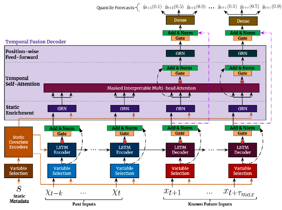
The first TFT’s step is embed the original input {x(s),x(h),x(f)}\{\mathbf{x}^{(s)}, \mathbf{x}^{(h)}, \mathbf{x}^{(f)}\} into a high dimensional space {E(s),E(h),E(f)}\{\mathbf{E}^{(s)}, \mathbf{E}^{(h)}, \mathbf{E}^{(f)}\}, after which each embedding is gated by a variable selection network (VSN). The static embedding E(s)\mathbf{E}^{(s)} is used as context for variable selection and as initial condition to the LSTM. Finally the encoded variables are fed into the multi-head attention decoder.

2.1 Static Covariate Encoder

The static embedding E(s)\mathbf{E}^{(s)} is transformed by the StaticCovariateEncoder into contexts cs,ce,ch,ccc_{s}, c_{e}, c_{h}, c_{c}. Where csc_{s} are temporal variable selection contexts, cec_{e} are TemporalFusionDecoder enriching contexts, and ch,ccc_{h}, c_{c} are LSTM’s hidden/contexts for the TemporalCovariateEncoder.

2.2 Temporal Covariate Encoder

TemporalCovariateEncoder encodes the embeddings E(h),E(f)\mathbf{E}^{(h)}, \mathbf{E}^{(f)} and contexts (ch,cc)(c_{h}, c_{c}) with an LSTM. An analogous process is repeated for the future data, with the main difference that E(f)\mathbf{E}^{(f)} contains the future available information.

2.3 Temporal Fusion Decoder

The TemporalFusionDecoder enriches the LSTM’s outputs with cec_{e} and then uses an attention layer, and multi-step adapter.

3. Interpretability

3.1 Attention Weights

attention = nf.models[0].attention_weights()
def plot_attention(
    self, plot: str = "time", output: str = "plot", width: int = 800, height: int = 400
):
    """
    Plot the attention weights.

    Args:
        plot (str, optional): The type of plot to generate. Can be one of the following:
            - 'time': Display the mean attention weights over time.
            - 'all': Display the attention weights for each horizon.
            - 'heatmap': Display the attention weights as a heatmap.
            - An integer in the range [1, model.h) to display the attention weights for a specific horizon.
        output (str, optional): The type of output to generate. Can be one of the following:
            - 'plot': Display the plot directly.
            - 'figure': Return the plot as a figure object.
        width (int, optional): Width of the plot in pixels. Default is 800.
        height (int, optional): Height of the plot in pixels. Default is 400.

    Returns:
        matplotlib.figure.Figure: If `output` is 'figure', the function returns the plot as a figure object.
    """

    attention = (
        self.mean_on_batch(self.interpretability_params["attn_wts"])
        .mean(dim=0)
        .cpu()
        .numpy()
    )

    fig, ax = plt.subplots(figsize=(width / 100, height / 100))

    if plot == "time":
        attention = attention[self.input_size :, :].mean(axis=0)
        ax.plot(np.arange(-self.input_size, self.h), attention)
        ax.axvline(
            x=0, color="black", linewidth=3, linestyle="--", label="prediction start"
        )
        ax.set_title("Mean Attention")
        ax.set_xlabel("time")
        ax.set_ylabel("Attention")
        ax.legend()

    elif plot == "all":
        for i in range(self.input_size, attention.shape[0]):
            ax.plot(
                np.arange(-self.input_size, self.h),
                attention[i, :],
                label=f"horizon {i-self.input_size+1}",
            )
        ax.axvline(
            x=0, color="black", linewidth=3, linestyle="--", label="prediction start"
        )
        ax.set_title("Attention per horizon")
        ax.set_xlabel("time")
        ax.set_ylabel("Attention")
        ax.legend()

    elif plot == "heatmap":
        cax = ax.imshow(
            attention,
            aspect="auto",
            cmap="viridis",
            extent=[-self.input_size, self.h, -self.input_size, self.h],
        )
        fig.colorbar(cax)
        ax.set_title("Attention Heatmap")
        ax.set_xlabel("Attention (current time step)")
        ax.set_ylabel("Attention (previous time step)")

    elif isinstance(plot, int) and (plot in np.arange(1, self.h + 1)):
        i = self.input_size + plot - 1
        ax.plot(
            np.arange(-self.input_size, self.h),
            attention[i, :],
            label=f"horizon {plot}",
        )
        ax.axvline(
            x=0, color="black", linewidth=3, linestyle="--", label="prediction start"
        )
        ax.set_title(f"Attention weight for horizon {plot}")
        ax.set_xlabel("time")
        ax.set_ylabel("Attention")
        ax.legend()

    else:
        raise ValueError(
            'plot has to be in ["time","all","heatmap"] or integer in range(1,model.h)'
        )

    plt.tight_layout()

    if output == "plot":
        plt.show()
    elif output == "figure":
        return fig
    else:
        raise ValueError(f"Invalid output: {output}. Expected 'plot' or 'figure'.")
3.1.1 Mean attention
plot_attention(nf.models[0], plot="time")
3.1.2 Attention of all future time steps
plot_attention(nf.models[0], plot="all")
3.1.3 Attention of a specific future time step
plot_attention(nf.models[0], plot=8)

3.2 Feature Importance

3.2.1 Global feature importance

feature_importances = nf.models[0].feature_importances()
feature_importances.keys()
Static variable importances
feature_importances["Static covariates"].sort_values(by="importance").plot(kind="barh")
Past variable importances
feature_importances["Past variable importance over time"].mean().sort_values().plot(
    kind="barh"
)
Future variable importances
feature_importances["Future variable importance over time"].mean().sort_values().plot(
    kind="barh"
)

3.2.2 Variable importances over time

Future variable importance over time
Importance of each future covariate at each future time step
df = feature_importances["Future variable importance over time"]


fig, ax = plt.subplots(figsize=(20, 10))
bottom = np.zeros(len(df.index))
for col in df.columns:
    p = ax.bar(np.arange(-len(df), 0), df[col].values, 0.6, label=col, bottom=bottom)
    bottom += df[col]
ax.set_title("Future variable importance over time ponderated by attention")
ax.set_ylabel("Importance")
ax.set_xlabel("Time")
ax.grid(True)
ax.legend()
plt.show()
Past variable importance over time
df = feature_importances["Past variable importance over time"]

fig, ax = plt.subplots(figsize=(20, 10))
bottom = np.zeros(len(df.index))

for col in df.columns:
    p = ax.bar(np.arange(-len(df), 0), df[col].values, 0.6, label=col, bottom=bottom)
    bottom += df[col]
ax.set_title("Past variable importance over time")
ax.set_ylabel("Importance")
ax.set_xlabel("Time")
ax.legend()
ax.grid(True)

plt.show()
Past variable importance over time ponderated by attention
Decomposition of the importance of each time step based on importance of each variable at that time step
df = feature_importances["Past variable importance over time"]
mean_attention = (
    nf.models[0]
    .attention_weights()[nf.models[0].input_size :, :]
    .mean(axis=0)[: nf.models[0].input_size]
)
df = df.multiply(mean_attention, axis=0)

fig, ax = plt.subplots(figsize=(20, 10))
bottom = np.zeros(len(df.index))

for col in df.columns:
    p = ax.bar(np.arange(-len(df), 0), df[col].values, 0.6, label=col, bottom=bottom)
    bottom += df[col]
ax.set_title("Past variable importance over time ponderated by attention")
ax.set_ylabel("Importance")
ax.set_xlabel("Time")
ax.legend()
ax.grid(True)
plt.plot(
    np.arange(-len(df), 0),
    mean_attention,
    color="black",
    marker="o",
    linestyle="-",
    linewidth=2,
    label="mean_attention",
)
plt.legend()
plt.show()

3.2.3 Variable importance correlations over time

Variables which gain and lose importance at same moments
nf.models[0].feature_importance_correlations()

4. Auxiliary Functions

4.1 Gating Mechanisms

The Gated Residual Network (GRN) provides adaptive depth and network complexity capable of accommodating different size datasets. As residual connections allow for the network to skip the non-linear transformation of input a\mathbf{a} and context c\mathbf{c}. The Gated Linear Unit (GLU) provides the flexibility of supressing unnecesary parts of the GRN. Consider GRN’s output γ\gamma then GLU transformation is defined by: GLU(γ)=σ(W4γ+b4)(W5γ+b5)\mathrm{GLU}(\gamma) = \sigma(\mathbf{W}_{4}\gamma +b_{4}) \odot (\mathbf{W}_{5}\gamma +b_{5}) Figure 2. Gated Residual Network. Figure 2. Gated Residual Network.

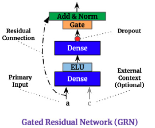
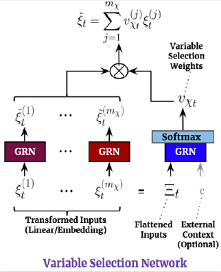
4.2 Variable Selection Networks

TFT includes automated variable selection capabilities, through its variable selection network (VSN) components. The VSN takes the original input {x(s),x[:t](h),x[:t](f)}\{\mathbf{x}^{(s)}, \mathbf{x}^{(h)}_{[:t]}, \mathbf{x}^{(f)}_{[:t]}\} and transforms it through embeddings or linear transformations into a high dimensional space {E(s),E[:t](h),E[:t+H](f)}\{\mathbf{E}^{(s)}, \mathbf{E}^{(h)}_{[:t]}, \mathbf{E}^{(f)}_{[:t+H]}\}. For the observed historic data, the embedding matrix Et(h)\mathbf{E}^{(h)}_{t} at time tt is a concatenation of jj variable et,j(h)e^{(h)}_{t,j} embeddings: The variable selection weights are given by: st(h)=SoftMax(GRN(Et(h),E(s)))s^{(h)}_{t}=\mathrm{SoftMax}(\mathrm{GRN}(\mathbf{E}^{(h)}_{t},\mathbf{E}^{(s)})) The VSN processed features are then: E~t(h)=jsj(h)e~t,j(h)\tilde{\mathbf{E}}^{(h)}_{t}= \sum_{j} s^{(h)}_{j} \tilde{e}^{(h)}_{t,j} Figure 3. Variable Selection Network Figure 3. Variable Selection Network

4.3. Multi-Head Attention

To avoid information bottlenecks from the classic Seq2Seq architecture, TFT incorporates a decoder-encoder attention mechanism inherited transformer architectures (Li et. al 2019, Vaswani et. al 2017). It transform the the outputs of the LSTM encoded temporal features, and helps the decoder better capture long-term relationships. The original multihead attention for each component HmH_{m} and its query, key, and value representations are denoted by Qm,Km,VmQ_{m}, K_{m}, V_{m}, its transformation is given by: TFT modifies the original multihead attention to improve its interpretability. To do it it uses shared values V~\tilde{V} across heads and employs additive aggregation, InterpretableMultiHead(Q,K,V)=H~WM\mathrm{InterpretableMultiHead}(Q,K,V) = \tilde{H} W_{M}. The mechanism has a great resemblence to a single attention layer, but it allows for MM multiple attention weights, and can be therefore be interpreted as the average ensemble of MM single attention layers.