Hyperparameter Optimization | NeuralForecast

Deep-learning models are the state-of-the-art in time series forecasting. They have outperformed statistical and tree-based approaches in recent large-scale competitions, such as the M series, and are being increasingly adopted in industry. However, their performance is greatly affected by the choice of hyperparameters. Selecting the optimal configuration, a process called hyperparameter tuning, is essential to achieve the best performance. The main steps of hyperparameter tuning are:

Define training and validation sets.
Define search space.
Sample configurations with a search algorithm, train models, and evaluate them on the validation set.
Select and store the best model.

With Neuralforecast, we automatize and simplify the hyperparameter tuning process with the Auto models. Every model in the library has an Auto version (for example, AutoNHITS, AutoTFT) which can perform automatic hyperparameter selection on default or user-defined search space. The Auto models can be used with two backends: Ray’s Tune library and Optuna, with a user-friendly and simplified API, with most of their capabilities. In this tutorial, we show in detail how to instantiate and train an AutoNHITS model with a custom search space with both Tune and Optuna backends, install and use HYPEROPT search algorithm, and use the model with optimal hyperparameters to forecast. You can run these experiments using GPU with Google Colab.

1. Install `Neuralforecast`

%%capture
!pip install neuralforecast hyperopt

2. Load Data

In this example we will use the AirPasengers, a popular dataset with monthly airline passengers in the US from 1949 to 1960. Load the data, available at our utils methods in the required format. See https://nixtlaverse.nixtla.io/neuralforecast/utils.html#example-data for more details on the data input format.

import logging

from neuralforecast.utils import AirPassengersDF

logging.getLogger('pytorch_lightning').setLevel(logging.ERROR)

Y_df = AirPassengersDF
Y_df.head()

	unique_id	ds	y
0	1.0	1949-01-31	112.0
1	1.0	1949-02-28	118.0
2	1.0	1949-03-31	132.0
3	1.0	1949-04-30	129.0
4	1.0	1949-05-31	121.0

3. Ray’s `Tune` backend

First, we show how to use the Tune backend. This backend is based on Ray’s Tune library, which is a scalable framework for hyperparameter tuning. It is a popular library in the machine learning community, and it is used by many companies and research labs. If you plan to use the Optuna backend, you can skip this section.

3.a Define hyperparameter grid

Each Auto model contains a default search space that was extensively tested on multiple large-scale datasets. Search spaces are specified with dictionaries, where keys corresponds to the model’s hyperparameter and the value is a Tune function to specify how the hyperparameter will be sampled. For example, use randint to sample integers uniformly, and choice to sample values of a list.

3.a.1 Default hyperparameter grid

The default search space dictionary can be accessed through the get_default_config function of the Auto model. This is useful if you wish to use the default parameter configuration but want to change one or more hyperparameter spaces without changing the other default values. To extract the default config, you need to define: * h: forecasting horizon. * backend: backend to use. * n_series: Optional, the number of unique time series, required only for Multivariate models. In this example, we will use h=12 and we use ray as backend. We will use the default hyperparameter space but only change random_seed range and n_pool_kernel_size.

from ray import tune
from neuralforecast.auto import AutoNHITS

nhits_config = AutoNHITS.get_default_config(h = 12, backend="ray")                      # Extract the default hyperparameter settings
nhits_config["random_seed"] = tune.randint(1, 10)                                       # Random seed
nhits_config["n_pool_kernel_size"] = tune.choice([[2, 2, 2], [16, 8, 1]])               # MaxPool's Kernelsize

3.a.2 Custom hyperparameter grid

More generally, users can define fully customized search spaces tailored for particular datasets and tasks, by fully specifying a hyperparameter search space dictionary. In the following example we are optimizing the learning_rate and two NHITS specific hyperparameters: n_pool_kernel_size and n_freq_downsample. Additionaly, we use the search space to modify default hyperparameters, such as max_steps and val_check_steps.

nhits_config = {
   "max_steps": 100,                                                         # Number of SGD steps
   "input_size": 24,                                                         # Size of input window
   "learning_rate": tune.loguniform(1e-5, 1e-1),                             # Initial Learning rate
   "n_pool_kernel_size": tune.choice([[2, 2, 2], [16, 8, 1]]),               # MaxPool's Kernelsize
   "n_freq_downsample": tune.choice([[168, 24, 1], [24, 12, 1], [1, 1, 1]]), # Interpolation expressivity ratios
   "val_check_steps": 50,                                                    # Compute validation every 50 steps
   "random_seed": tune.randint(1, 10),                                       # Random seed
}

Important Configuration dictionaries are not interchangeable between models since they have different hyperparameters. Refer to https://nixtlaverse.nixtla.io/neuralforecast/models.html for a complete list of each model’s hyperparameters.

3.b Instantiate `Auto` model

To instantiate an Auto model you need to define:

h: forecasting horizon.
loss: training and validation loss from neuralforecast.losses.pytorch.
config: hyperparameter search space. If None, the Auto class will use a pre-defined suggested hyperparameter space.
search_alg: search algorithm (from tune.search), default is random search. Refer to https://docs.ray.io/en/latest/tune/api_docs/suggestion.html for more information on the different search algorithm options.
backend: backend to use, default is ray. If optuna, the Auto class will use the Optuna backend.
num_samples: number of configurations explored.

In this example we set horizon h as 12, use the MAE loss for training and validation, and use the HYPEROPT search algorithm.

from ray.tune.search.hyperopt import HyperOptSearch
from neuralforecast.losses.pytorch import MAE
from neuralforecast.auto import AutoNHITS

model = AutoNHITS(
    h=12,
    loss=MAE(),
    config=nhits_config,
    search_alg=HyperOptSearch(),
    backend='ray',
    num_samples=10,
)

Tip The number of samples, num_samples, is a crucial parameter! Larger values will usually produce better results as we explore more configurations in the search space, but it will increase training times. Larger search spaces will usually require more samples. As a general rule, we recommend setting num_samples higher than 20. We set 10 in this example for demonstration purposes.

3.c Train model and predict with `Core` class

Next, we use the Neuralforecast class to train the Auto model. In this step, Auto models will automatically perform hyperparamter tuning training multiple models with different hyperparameters, producing the forecasts on the validation set, and evaluating them. The best configuration is selected based on the error on a validation set. Only the best model is stored and used during inference.

from neuralforecast import NeuralForecast

Use the val_size parameter of the fit method to control the length of the validation set. In this case we set the validation set as twice the forecasting horizon.

%%capture
nf = NeuralForecast(models=[model], freq='ME')
nf.fit(df=Y_df, val_size=24)

The results of the hyperparameter tuning are available in the results attribute of the Auto model. Use the get_dataframe method to get the results in a pandas dataframe.

results = nf.models[0].results.get_dataframe()
results.head()

	loss	train_loss	timestamp	checkpoint_dir_name	done	training_iteration	trial_id	date	time_this_iter_s	time_total_s	…	config/input_size	config/learning_rate	config/n_pool_kernel_size	config/n_freq_downsample	config/val_check_steps	config/random_seed	config/h	config/loss	config/valid_loss	logdir
0	21.948565	11.748630	1732660404	None	False	2	e684ab59	2024-11-26_22-33-24	0.473169	1.742914	…	24	0.000583	(16, 8, 1)	(1, 1, 1)	50	9	12	MAE()	MAE()	e684ab59
1	23.497557	13.491600	1732660411	None	False	2	28016d96	2024-11-26_22-33-31	0.467711	1.767644	…	24	0.000222	(16, 8, 1)	(168, 24, 1)	50	5	12	MAE()	MAE()	28016d96
2	29.214516	16.968582	1732660419	None	False	2	ded66a42	2024-11-26_22-33-39	0.969751	2.623766	…	24	0.009816	(16, 8, 1)	(24, 12, 1)	50	5	12	MAE()	MAE()	ded66a42
3	45.178616	28.338690	1732660427	None	False	2	2964d41f	2024-11-26_22-33-47	0.985556	2.656381	…	24	0.012083	(16, 8, 1)	(24, 12, 1)	50	7	12	MAE()	MAE()	2964d41f
4	32.580570	21.667740	1732660434	None	False	2	766cc549	2024-11-26_22-33-54	0.418154	1.465539	…	24	0.000040	(2, 2, 2)	(1, 1, 1)	50	4	12	MAE()	MAE()	766cc549

Next, we use the predict method to forecast the next 12 months using the optimal hyperparameters.

Y_hat_df = nf.predict()
Y_hat_df.head()

Predicting: |                                                                                                 …

	unique_id	ds	AutoNHITS
0	1.0	1961-01-31	438.724091
1	1.0	1961-02-28	415.593628
2	1.0	1961-03-31	493.484894
3	1.0	1961-04-30	493.120728
4	1.0	1961-05-31	499.806702

4. `Optuna` backend

In this section we show how to use the Optuna backend. Optuna is a lightweight and versatile platform for hyperparameter optimization. If you plan to use the Tune backend, you can skip this section.

4.a Define hyperparameter grid

Each Auto model contains a default search space that was extensively tested on multiple large-scale datasets. Search spaces are specified with a function that returns a dictionary, where keys corresponds to the model’s hyperparameter and the value is a suggest function to specify how the hyperparameter will be sampled. For example, use suggest_int to sample integers uniformly, and suggest_categorical to sample values of a list. See https://optuna.readthedocs.io/en/stable/reference/generated/optuna.trial.Trial.html for more details.

4.a.1 Default hyperparameter grid

The default search space dictionary can be accessed through the get_default_config function of the Auto model. This is useful if you wish to use the default parameter configuration but want to change one or more hyperparameter spaces without changing the other default values. To extract the default config, you need to define: * h: forecasting horizon. * backend: backend to use. * n_series: Optional, the number of unique time series, required only for Multivariate models. In this example, we will use h=12 and we use optuna as backend. We will use the default hyperparameter space but only change random_seed range and n_pool_kernel_size.

import optuna

optuna.logging.set_verbosity(optuna.logging.WARNING) # Use this to disable training prints from optuna
nhits_default_config = AutoNHITS.get_default_config(h = 12, backend="optuna")                   # Extract the default hyperparameter settings

def config_nhits(trial):
    config = {**nhits_default_config(trial)}
    config.update({
        "random_seed": trial.suggest_int("random_seed", 1, 10), 
        "n_pool_kernel_size": trial.suggest_categorical("n_pool_kernel_size", [[2, 2, 2], [16, 8, 1]])
    })
    return config    

3.a.2 Custom hyperparameter grid

More generally, users can define fully customized search spaces tailored for particular datasets and tasks, by fully specifying a hyperparameter search space function. In the following example we are optimizing the learning_rate and two NHITS specific hyperparameters: n_pool_kernel_size and n_freq_downsample. Additionaly, we use the search space to modify default hyperparameters, such as max_steps and val_check_steps.

def config_nhits(trial):
    return {
        "max_steps": 100,                                                                                               # Number of SGD steps
        "input_size": 24,                                                                                               # Size of input window
        "learning_rate": trial.suggest_loguniform("learning_rate", 1e-5, 1e-1),                                         # Initial Learning rate
        "n_pool_kernel_size": trial.suggest_categorical("n_pool_kernel_size", [[2, 2, 2], [16, 8, 1]]),                 # MaxPool's Kernelsize
        "n_freq_downsample": trial.suggest_categorical("n_freq_downsample", [[168, 24, 1], [24, 12, 1], [1, 1, 1]]),    # Interpolation expressivity ratios
        "val_check_steps": 50,                                                                                          # Compute validation every 50 steps
        "random_seed": trial.suggest_int("random_seed", 1, 10),                                                         # Random seed
    }

4.b Instantiate `Auto` model

To instantiate an Auto model you need to define:

h: forecasting horizon.
loss: training and validation loss from neuralforecast.losses.pytorch.
config: hyperparameter search space. If None, the Auto class will use a pre-defined suggested hyperparameter space.
search_alg: search algorithm (from optuna.samplers), default is TPESampler (Tree-structured Parzen Estimator). Refer to https://optuna.readthedocs.io/en/stable/reference/samplers/index.html for more information on the different search algorithm options.
backend: backend to use, default is ray. If optuna, the Auto class will use the Optuna backend.
num_samples: number of configurations explored.

model = AutoNHITS(
    h=12,
    loss=MAE(),
    config=config_nhits,
    search_alg=optuna.samplers.TPESampler(seed=0),
    backend='optuna',
    num_samples=10,
)

Important Configuration dictionaries and search algorithms for Tune and Optuna are not interchangeable! Use the appropriate type of search algorithm and custom configuration dictionary for each backend.

4.c Train model and predict with `Core` class

Use the val_size parameter of the fit method to control the length of the validation set. In this case we set the validation set as twice the forecasting horizon.

%%capture
nf = NeuralForecast(models=[model], freq='ME')
nf.fit(df=Y_df, val_size=24)

The results of the hyperparameter tuning are available in the results attribute of the Auto model. Use the trials_dataframe method to get the results in a pandas dataframe.

results = nf.models[0].results.trials_dataframe()
results.drop(columns='user_attrs_ALL_PARAMS')

	number	value	datetime_start	datetime_complete	duration	params_learning_rate	params_n_freq_downsample	params_n_pool_kernel_size	params_random_seed	user_attrs_METRICS	state
0	0	1.827570e+01	2024-11-26 22:34:29.382448	2024-11-26 22:34:30.773811	0 days 00:00:01.391363	0.001568	[1, 1, 1]	[2, 2, 2]	5	{‘loss’: tensor(18.2757), ‘train_loss’: tensor…	COMPLETE
1	1	9.055198e+06	2024-11-26 22:34:30.774153	2024-11-26 22:34:32.090132	0 days 00:00:01.315979	0.036906	[168, 24, 1]	[2, 2, 2]	10	{‘loss’: tensor(9055198.), ‘train_loss’: tenso…	COMPLETE
2	2	5.554298e+01	2024-11-26 22:34:32.090466	2024-11-26 22:34:33.425103	0 days 00:00:01.334637	0.000019	[1, 1, 1]	[2, 2, 2]	10	{‘loss’: tensor(55.5430), ‘train_loss’: tensor…	COMPLETE
3	3	9.857751e+01	2024-11-26 22:34:33.425460	2024-11-26 22:34:34.962057	0 days 00:00:01.536597	0.015727	[24, 12, 1]	[16, 8, 1]	10	{‘loss’: tensor(98.5775), ‘train_loss’: tensor…	COMPLETE
4	4	1.966841e+01	2024-11-26 22:34:34.962357	2024-11-26 22:34:36.951450	0 days 00:00:01.989093	0.001223	[168, 24, 1]	[2, 2, 2]	1	{‘loss’: tensor(19.6684), ‘train_loss’: tensor…	COMPLETE
5	5	1.524971e+01	2024-11-26 22:34:36.951775	2024-11-26 22:34:38.280982	0 days 00:00:01.329207	0.002955	[168, 24, 1]	[16, 8, 1]	5	{‘loss’: tensor(15.2497), ‘train_loss’: tensor…	COMPLETE
6	6	1.678810e+01	2024-11-26 22:34:38.281381	2024-11-26 22:34:39.648595	0 days 00:00:01.367214	0.006173	[168, 24, 1]	[16, 8, 1]	4	{‘loss’: tensor(16.7881), ‘train_loss’: tensor…	COMPLETE
7	7	2.014485e+01	2024-11-26 22:34:39.649025	2024-11-26 22:34:41.075568	0 days 00:00:01.426543	0.000285	[168, 24, 1]	[2, 2, 2]	2	{‘loss’: tensor(20.1448), ‘train_loss’: tensor…	COMPLETE
8	8	2.109382e+01	2024-11-26 22:34:41.075891	2024-11-26 22:34:42.449451	0 days 00:00:01.373560	0.004097	[168, 24, 1]	[16, 8, 1]	7	{‘loss’: tensor(21.0938), ‘train_loss’: tensor…	COMPLETE
9	9	5.091650e+01	2024-11-26 22:34:42.449762	2024-11-26 22:34:43.804981	0 days 00:00:01.355219	0.000036	[1, 1, 1]	[16, 8, 1]	1	{‘loss’: tensor(50.9165), ‘train_loss’: tensor…	COMPLETE

Next, we use the predict method to forecast the next 12 months using the optimal hyperparameters.

Y_hat_df_optuna = nf.predict()
Y_hat_df_optuna.head()

Predicting: |                                                                                                 …

	unique_id	ds	AutoNHITS
0	1.0	1961-01-31	446.410736
1	1.0	1961-02-28	422.048523
2	1.0	1961-03-31	508.271515
3	1.0	1961-04-30	496.549133
4	1.0	1961-05-31	506.865723

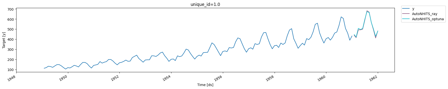
5. Plots

Finally, we compare the forecasts produced by the AutoNHITS model with both backends.

from utilsforecast.plotting import plot_series

plot_series(
    Y_df,
    Y_hat_df.merge(
        Y_hat_df_optuna,
        on=['unique_id', 'ds'],
        suffixes=['_ray', '_optuna'],
    ),
)

Getting Started

Capabilities

Tutorials

Use cases

API Reference

Hyperparameter Optimization | NeuralForecast

1. Install `Neuralforecast`

2. Load Data

3. Ray’s `Tune` backend

3.a Define hyperparameter grid

3.a.1 Default hyperparameter grid

3.a.2 Custom hyperparameter grid

3.b Instantiate `Auto` model

3.c Train model and predict with `Core` class

4. `Optuna` backend

4.a Define hyperparameter grid

4.a.1 Default hyperparameter grid

3.a.2 Custom hyperparameter grid

4.b Instantiate `Auto` model

4.c Train model and predict with `Core` class

5. Plots

References

Getting Started

Capabilities

Tutorials

Use cases

API Reference

Documentation Index

​1. Install Neuralforecast

​2. Load Data

​3. Ray’s Tune backend

​3.a Define hyperparameter grid

​3.a.1 Default hyperparameter grid

​3.a.2 Custom hyperparameter grid

​3.b Instantiate Auto model

​3.c Train model and predict with Core class

​4. Optuna backend

​4.a Define hyperparameter grid

​4.a.1 Default hyperparameter grid

​3.a.2 Custom hyperparameter grid

​4.b Instantiate Auto model

​4.c Train model and predict with Core class

​5. Plots

​References

1. Install `Neuralforecast`

2. Load Data

3. Ray’s `Tune` backend

3.a Define hyperparameter grid

3.a.1 Default hyperparameter grid

3.a.2 Custom hyperparameter grid

3.b Instantiate `Auto` model

3.c Train model and predict with `Core` class

4. `Optuna` backend

4.a Define hyperparameter grid

4.a.1 Default hyperparameter grid

3.a.2 Custom hyperparameter grid

4.b Instantiate `Auto` model

4.c Train model and predict with `Core` class

5. Plots

References

- Cristian Challu, Kin G. Olivares, Boris N. Oreshkin, Federico Garza, Max Mergenthaler-Canseco, Artur Dubrawski (2021). NHITS: Neural Hierarchical Interpolation for Time Series Forecasting. Accepted at AAAI 2023.
- James Bergstra, Remi Bardenet, Yoshua Bengio, and Balazs Kegl (2011). “Algorithms for Hyper-Parameter Optimization”. In: Advances in Neural Information Processing Systems. url: https://proceedings.neurips.cc/paper/2011/file/86e8f7ab32cfd12577bc2619bc635690-Paper.pdf
- Kirthevasan Kandasamy, Karun Raju Vysyaraju, Willie Neiswanger, Biswajit Paria, Christopher R. Collins, Jeff Schneider, Barnabas Poczos, Eric P. Xing (2019). “Tuning Hyperparameters without Grad Students: Scalable and Robust Bayesian Optimisation with Dragonfly”. Journal of Machine Learning Research. url: https://arxiv.org/abs/1903.06694
- Lisha Li, Kevin Jamieson, Giulia DeSalvo, Afshin Rostamizadeh, Ameet Talwalkar (2016). “Hyperband: A Novel Bandit-Based Approach to Hyperparameter Optimization”. Journal of Machine Learning Research. url: https://arxiv.org/abs/1603.06560