

Prerequesites This Guide assumes basic familiarity with NeuralForecast. For a minimal example visit the Quick StartTo measure the performance of a forecasting model, we can assess its performance on historical data using cross-validation. Cross-validation is done by defining a sliding window of input data to predict the following period. We do this operation many times such that the model predicts new periods, resulting in a more robust assessment of its performance. Below, you can see an illustration of cross-validation. In this illustration, the cross-validation process generates six different forecasting periods where we can compare the model’s predictions against the actual values of the past.
 This mimicks the process of making predictions in the future and
collecting actual data to then evaluate the prediction’s accuracy.
In this tutorial, we explore in detail the cross-validation function in
This mimicks the process of making predictions in the future and
collecting actual data to then evaluate the prediction’s accuracy.
In this tutorial, we explore in detail the cross-validation function in
neuralforecast.
1. Libraries
Make sure to installneuralforecast to follow along.
2. Read the data
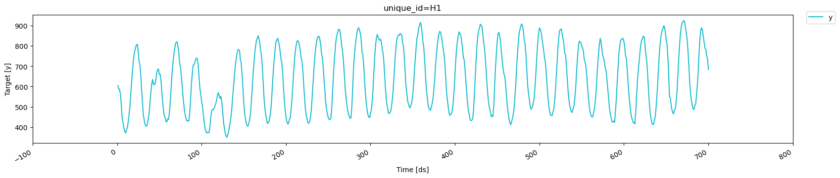
For this tutorial, we use part of the hourly M4 dataset. It is stored in a parquet file for efficiency. However, you can use ordinary pandas operations to read your data in other formats likes.csv.
The input to NeuralForecast is always a data frame in long
format with
three columns: unique_id, ds and y:
-
The
unique_id(string, int or category) represents an identifier for the series. -
The
ds(datestamp or int) column should be either an integer indexing time or a datestampe ideally like YYYY-MM-DD for a date or YYYY-MM-DD HH:MM:SS for a timestamp. -
The
y(numeric) represents the measurement we wish to forecast.
| unique_id | ds | y | |
|---|---|---|---|
| 0 | H1 | 1 | 605.0 |
| 1 | H1 | 2 | 586.0 |
| 2 | H1 | 3 | 586.0 |
| 3 | H1 | 4 | 559.0 |
| 4 | H1 | 5 | 511.0 |
| unique_id | ds | y | |
|---|---|---|---|
| 0 | H1 | 1 | 605.0 |
| 1 | H1 | 2 | 586.0 |
| 2 | H1 | 3 | 586.0 |
| 3 | H1 | 4 | 559.0 |
| 4 | H1 | 5 | 511.0 |
3. Using cross-validation
3.1 Using n_windows
To use the cross_validation method, we can either: - Set the sizes of
a validation and test set - Set a number of cross-validation windows
Let’s see how it works in a minimal example. Here, we use the NHITS
model and set the horizon to 100, and give an input size of 200.
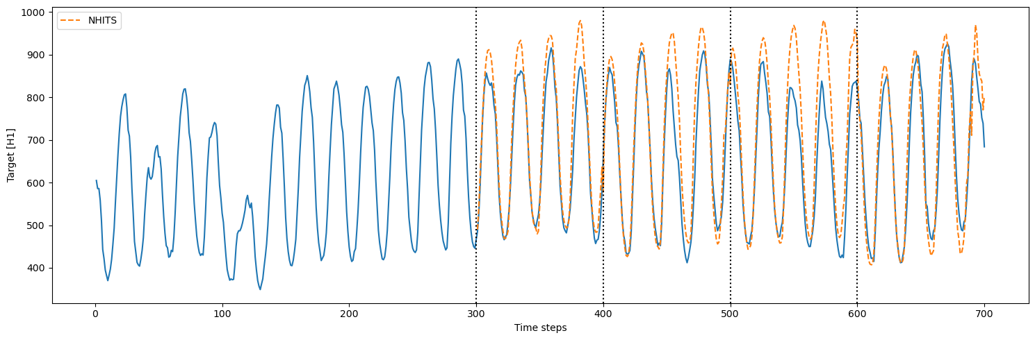
First, let’s use n_windows = 4.
We also set step_size equal to the horizon. This parameter controls
the distance between each cross-validation window. By setting it equal
to the horizon, we perform chained cross-validation where the windows
do not overlap.
| unique_id | ds | cutoff | NHITS | y | |
|---|---|---|---|---|---|
| 0 | H1 | 301 | 300 | 490.048950 | 485.0 |
| 1 | H1 | 302 | 300 | 537.713867 | 525.0 |
| 2 | H1 | 303 | 300 | 612.900635 | 585.0 |
| 3 | H1 | 304 | 300 | 689.346313 | 670.0 |
| 4 | H1 | 305 | 300 | 760.153992 | 747.0 |
Important note We start counting at 0, so counting from 0 to 99 results in a sequence of 100 data points.Thus, the model is initially trained using time steps 0 to 299. Then, to make predictions, it takes time steps 100 to 299 (input size of 200) and it makes predictions for time steps 300 to 399 (horizon of 100). Then, the actual values from 200 to 399 (because our model has an
input_size of 200) are used to generate predictions over the next
window, from 400 to 499.
This process is repeated until we run out of windows.
3.2 Using a validation and test set
Instead of setting a number of windows, we can define a validation and test set. In that case, we must setn_windows=None
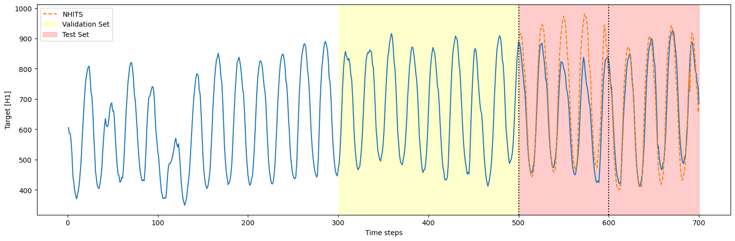
step_size is also set to 100, there are only two cross-validation
windows in the test set (200/100 = 2). Thus, we only see two cutoff
points.
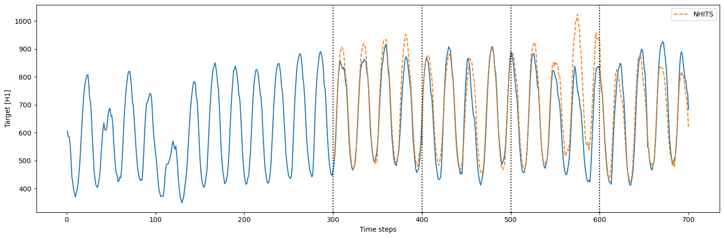
3.3 Cross-validation with refit
In the previous sections, we trained the model only once and predicted over many cross-validation windows. However, in real life, we often retrain our model with new observed data before making the next set of predictions. We can simulate that process usingrefit=True. That way, the model is
retrained at every step in the cross-validation process. In other words,
the training set is gradually expanded with new observed values and the
model is retrained before making the next set of predictions.
refit=True, there were 4
training loops that were completed. This is expected because the model
is now retrained with new data for each fold in the cross-validation: -
fold 1: train on the first 300 steps, predict the next 100 - fold 2:
train on the first 400 steps, predict the next 100 - fold 3: train on
the first 500 steps, predict the next 100 - fold 4: train on the first
600 steps, predict the next 100
3.4 Overlapping windows in cross-validation
In the case wherestep_size is smaller than the horizon, we get
overlapping windows. This means that we make predictions more than once
for some time steps.
This is useful to test the model over more forecast windows, and it
provides a more robust evaluation, as the model is tested across
different segments of the series.
However, it comes with a higher computation cost, as we are making
predictions more than once for some of the time steps.
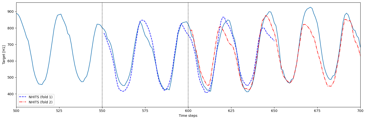
- fold 1: model is trained using time steps 0 to 550 and predicts 551 to 650 (h=100)
- fold 2: model is trained using time steps 0 to 600 (
step_size=50) and predicts 601 to 700