

In this example we will show how to perform electricity load forecasting considering a model capable of handling multiple seasonalities (MSTL).
Introduction
Some time series are generated from very low frequency data. These data generally exhibit multiple seasonalities. For example, hourly data may exhibit repeated patterns every hour (every 24 observations) or every day (every 24 * 7, hours per day, observations). This is the case for electricity load. Electricity load may vary hourly, e.g., during the evenings electricity consumption may be expected to increase. But also, the electricity load varies by week. Perhaps on weekends there is an increase in electrical activity. In this example we will show how to model the two seasonalities of the time series to generate accurate forecasts in a short time. We will use hourly PJM electricity load data. The original data can be found here.Libraries
In this example we will use the following libraries:StatsForecast. Lightning ⚡️ fast forecasting with statistical and econometric models. Includes the MSTL model for multiple seasonalities.Prophet. Benchmark model developed by Facebook.NeuralProphet. Deep Learning version ofProphet. Used as benchark.
Forecast using Multiple Seasonalities
Electricity Load Data
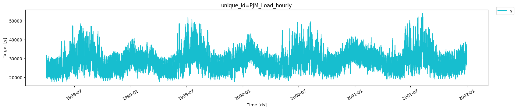
According to the dataset’s page,PJM Interconnection LLC (PJM) is a regional transmission organization (RTO) in the United States. It is part of the Eastern Interconnection grid operating an electric transmission system serving all or parts of Delaware, Illinois, Indiana, Kentucky, Maryland, Michigan, New Jersey, North Carolina, Ohio, Pennsylvania, Tennessee, Virginia, West Virginia, and the District of Columbia. The hourly power consumption data comes from PJM’s website and are in megawatts (MW).Let’s take a look to the data.
| unique_id | ds | y | |
|---|---|---|---|
| 32891 | PJM_Load_hourly | 2001-12-31 20:00:00 | 36392.0 |
| 32892 | PJM_Load_hourly | 2001-12-31 21:00:00 | 35082.0 |
| 32893 | PJM_Load_hourly | 2001-12-31 22:00:00 | 33890.0 |
| 32894 | PJM_Load_hourly | 2001-12-31 23:00:00 | 32590.0 |
| 32895 | PJM_Load_hourly | 2002-01-01 00:00:00 | 31569.0 |
32,896 observations, so it is
necessary to use very computationally efficient methods to display them
in production.
MSTL model
The MSTL (Multiple Seasonal-Trend decomposition using LOESS) model, originally developed by Kasun Bandara, Rob J Hyndman and Christoph Bergmeir, decomposes the time series in multiple seasonalities using a Local Polynomial Regression (LOESS). Then it forecasts the trend using a custom non-seasonal model and each seasonality using a SeasonalNaive model.StatsForecast contains a fast implementation of the
MSTL model. Also,
the decomposition of the time series can be calculated.
[24, 24 * 7] as
the seasonalities that the
MSTL model receives.
We must also specify the manner in which the trend will be forecasted.
In this case we will use the
AutoARIMA model.
StatsForecast class to create forecasts.
Fit the model
Afer that, we just have to use thefit method to fit each model to
each time series.
Decompose the time series in multiple seasonalities
Once the model is fitted, we can access the decomposition using thefitted_ attribute of StatsForecast. This attribute stores all
relevant information of the fitted models for each of the time series.
In this case we are fitting a single model for a single time series, so
by accessing the fitted_ location [0, 0] we will find the relevant
information of our model. The MSTL
class generates a model_ attribute that contains the way the series
was decomposed.
| data | trend | seasonal24 | seasonal168 | remainder | |
|---|---|---|---|---|---|
| 0 | 22259.0 | 25899.808157 | -4720.213546 | 581.308595 | 498.096794 |
| 1 | 21244.0 | 25900.349395 | -5433.168901 | 571.780657 | 205.038849 |
| 2 | 20651.0 | 25900.875973 | -5829.135728 | 557.142643 | 22.117112 |
| 3 | 20421.0 | 25901.387631 | -5704.092794 | 597.696957 | -373.991794 |
| 4 | 20713.0 | 25901.884103 | -5023.324375 | 922.564854 | -1088.124582 |
| … | … | … | … | … | … |
| 32891 | 36392.0 | 33329.031577 | 4254.112720 | 917.258336 | -2108.402633 |
| 32892 | 35082.0 | 33355.083576 | 3625.077164 | 721.689136 | -2619.849876 |
| 32893 | 33890.0 | 33381.108409 | 2571.794472 | 549.661529 | -2612.564409 |
| 32894 | 32590.0 | 33407.105839 | 796.356548 | 361.956280 | -1975.418667 |
| 32895 | 31569.0 | 33433.075723 | -1260.860917 | 279.777069 | -882.991876 |
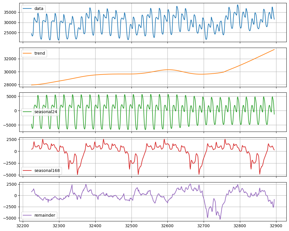
24 * 7 hours there is a very
well defined pattern. These two components will be forecast separately
using a SeasonalNaive model.
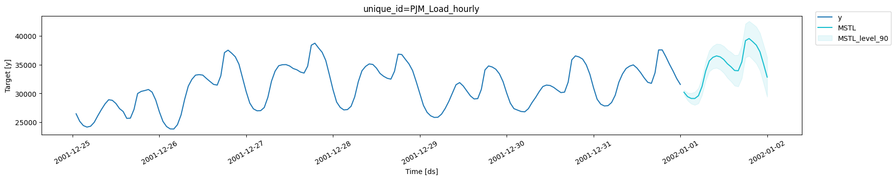
Produce forecasts
To generate forecasts we only have to use thepredict method
specifying the forecast horizon (h). In addition, to calculate
prediction intervals associated to the forecasts, we can include the
parameter level that receives a list of levels of the prediction
intervals we want to build. In this case we will only calculate the 90%
forecast interval (level=[90]).
| unique_id | ds | MSTL | MSTL-lo-90 | MSTL-hi-90 | |
|---|---|---|---|---|---|
| 0 | PJM_Load_hourly | 2002-01-01 01:00:00 | 30215.608163 | 29842.185622 | 30589.030705 |
| 1 | PJM_Load_hourly | 2002-01-01 02:00:00 | 29447.209028 | 28787.123369 | 30107.294687 |
| 2 | PJM_Load_hourly | 2002-01-01 03:00:00 | 29132.787603 | 28221.354454 | 30044.220751 |
| 3 | PJM_Load_hourly | 2002-01-01 04:00:00 | 29126.254591 | 27992.821420 | 30259.687762 |
| 4 | PJM_Load_hourly | 2002-01-01 05:00:00 | 29604.608674 | 28273.428663 | 30935.788686 |
Performance of the MSTL model
Split Train/Test sets
To validate the accuracy of theMSTL model, we will show its
performance on unseen data. We will use a classical time series
technique that consists of dividing the data into a training set and a
test set. We will leave the last 24 observations (the last day) as the
test set. So the model will train on 32,872 observations.
MSTL model
In addition to theMSTL model, we will include the
SeasonalNaive model as a
benchmark to validate the added value of the MSTL model. Including
StatsForecast models is as simple as adding them to the list of models
to be fitted.
time module.
| unique_id | ds | MSTL | MSTL-lo-90 | MSTL-hi-90 | SeasonalNaive | SeasonalNaive-lo-90 | SeasonalNaive-hi-90 | |
|---|---|---|---|---|---|---|---|---|
| 0 | PJM_Load_hourly | 2001-12-31 01:00:00 | 29158.872180 | 28785.567875 | 29532.176486 | 28326.0 | 23468.555872 | 33183.444128 |
| 1 | PJM_Load_hourly | 2001-12-31 02:00:00 | 28233.452263 | 27573.789089 | 28893.115438 | 27362.0 | 22504.555872 | 32219.444128 |
| 2 | PJM_Load_hourly | 2001-12-31 03:00:00 | 27915.251368 | 27004.459000 | 28826.043736 | 27108.0 | 22250.555872 | 31965.444128 |
| 3 | PJM_Load_hourly | 2001-12-31 04:00:00 | 27969.396560 | 26836.674164 | 29102.118956 | 26865.0 | 22007.555872 | 31722.444128 |
| 4 | PJM_Load_hourly | 2001-12-31 05:00:00 | 28469.805588 | 27139.306401 | 29800.304775 | 26808.0 | 21950.555872 | 31665.444128 |
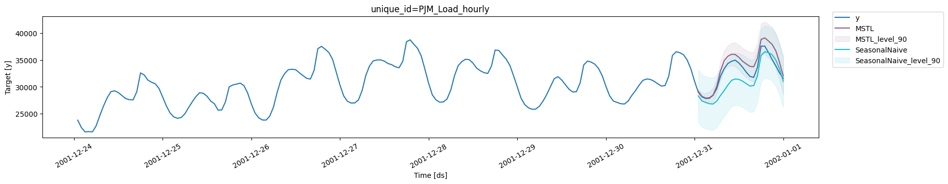
MSTL.
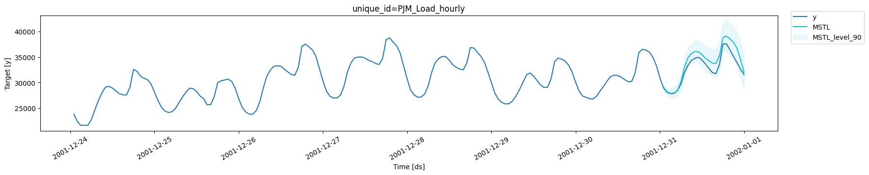
MSTL produces very accurate forecasts that follow the
behavior of the time series. Now let us calculate numerically the
accuracy of the model. We will use the following metrics: MAE, MAPE,
MASE, RMSE, SMAPE.
| metric | mase | mae | mape | rmse | smape |
|---|---|---|---|---|---|
| MSTL | 0.587265 | 1219.321795 | 0.036052 | 1460.223279 | 0.017577 |
| SeasonalNaive | 0.894653 | 1857.541667 | 0.056482 | 2201.384101 | 0.029343 |
MSTL has an improvement of about 35% over the
SeasonalNaive method in the test set measured in MASE.
Comparison with Prophet
One of the most widely used models for time series forecasting isProphet. This model is known for its ability to model different
seasonalities (weekly, daily yearly). We will use this model as a
benchmark to see if the MSTL adds value for this time series.
| unique_id | ds | Prophet | Prophet-lo-90 | Prophet-hi-90 | |
|---|---|---|---|---|---|
| 0 | PJM_Load_hourly | 2001-12-31 01:00:00 | 25294.246960 | 20299.105766 | 30100.467618 |
| 1 | PJM_Load_hourly | 2001-12-31 02:00:00 | 24000.725423 | 19285.395144 | 28777.495372 |
| 2 | PJM_Load_hourly | 2001-12-31 03:00:00 | 23324.771966 | 18536.736306 | 28057.063589 |
| 3 | PJM_Load_hourly | 2001-12-31 04:00:00 | 23332.519871 | 18591.879190 | 28720.461289 |
| 4 | PJM_Load_hourly | 2001-12-31 05:00:00 | 24107.126827 | 18934.471254 | 29116.352931 |
| model | time (mins) | |
|---|---|---|
| 0 | MSTL | 0.455999 |
| 1 | Prophet | 0.408726 |
Prophet to perform the fit and
predict pipeline is greater than MSTL. Let’s look at the forecasts
produced by Prophet.
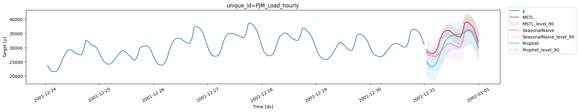
Prophet is able to capture the overall behavior of the
time series. However, in some cases it produces forecasts well below the
actual value. It also does not correctly adjust the valleys.
| metric | mase | mae | mape | rmse | smape |
|---|---|---|---|---|---|
| MSTL | 0.587265 | 1219.321795 | 0.036052 | 1460.223279 | 0.017577 |
| SeasonalNaive | 0.894653 | 1857.541667 | 0.056482 | 2201.384101 | 0.029343 |
| Prophet | 1.099551 | 2282.966977 | 0.073750 | 2721.817203 | 0.038633 |
Prophet is not able to produce better forecasts
than the SeasonalNaive model, however, the MSTL model improves
Prophet’s forecasts by 45% (MASE).
Comparison with NeuralProphet
NeuralProphet is the version of Prophet using deep learning. This
model is also capable of handling different seasonalities so we will
also use it as a benchmark.
| unique_id | ds | NeuralProphet | NeuralProphet-lo-90 | NeuralProphet-hi-90 | |
|---|---|---|---|---|---|
| 0 | PJM_Load_hourly | 2001-12-31 01:00:00 | 25292.386719 | 22520.238281 | 27889.425781 |
| 1 | PJM_Load_hourly | 2001-12-31 02:00:00 | 24378.796875 | 21640.460938 | 27056.906250 |
| 2 | PJM_Load_hourly | 2001-12-31 03:00:00 | 23852.919922 | 20978.291016 | 26583.130859 |
| 3 | PJM_Load_hourly | 2001-12-31 04:00:00 | 23540.554688 | 20700.035156 | 26247.121094 |
| 4 | PJM_Load_hourly | 2001-12-31 05:00:00 | 24016.589844 | 21298.316406 | 26748.933594 |
| model | time (mins) | |
|---|---|---|
| 0 | MSTL | 0.455999 |
| 1 | Prophet | 0.408726 |
| 0 | NeuralProphet | 1.981253 |
NeuralProphet requires a longer processing time than
Prophet and MSTL.
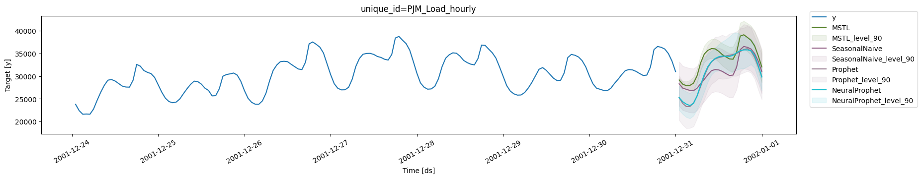
NeuralProphet generates very similar
results to Prophet, as expected.
| metric | mase | mae | mape | rmse | smape |
|---|---|---|---|---|---|
| MSTL | 0.587265 | 1219.321795 | 0.036052 | 1460.223279 | 0.017577 |
| SeasonalNaive | 0.894653 | 1857.541667 | 0.056482 | 2201.384101 | 0.029343 |
| Prophet | 1.099551 | 2282.966977 | 0.073750 | 2721.817203 | 0.038633 |
| NeuralProphet | 1.061160 | 2203.255941 | 0.071060 | 2593.708496 | 0.037108 |
NeuralProphet improves the
results of Prophet, as expected, however, MSTL improves over
NeuralProphet’s foreacasts by 44% (MASE).
Important
The performance of NeuralProphet can be improved using
hyperparameter optimization, which can increase the fitting time
significantly. In this example we show its performance with the
default version.
Conclusion
In this post we introducedMSTL, a model originally developed by
Kasun Bandara, Rob Hyndman and Christoph
Bergmeir capable of handling time
series with multiple seasonalities. We also showed that for the PJM
electricity load time series offers better performance in time and
accuracy than the Prophet and NeuralProphet models.