

In this notebook, we’ll incorporate exogenous regressors to a StatsForecast model.
Prerequisites This tutorial assumes basic familiarity with StatsForecast. For a minimal example visit the Quick Start
Introduction
Exogenous regressors are variables that can affect the values of a time series. They may not be directly related to the variable that is being forecasted, but they can still have an impact on it. Examples of exogenous regressors are weather data, economic indicators, or promotional sales. They are typically collected from external sources and by incorporating them into a forecasting model, they can improve the accuracy of our predictions. By the end of this tutorial, you’ll have a good understanding of how to incorporate exogenous regressors into StatsForecast’s models. Furthermore, you’ll see how to evaluate their performance and decide whether or not they can help enhance the forecast. Outline- Install libraries
- Load and explore the data
- Split train/test set
- Add exogenous regressors
- Create future exogenous regressors
- Train model
- Evaluate results
Tip You can use Colab to run this Notebook interactively
Install libraries
We assume that you have StatsForecast already installed. If not, check this guide for instructions on how to install StatsForecast.Load and explore the data
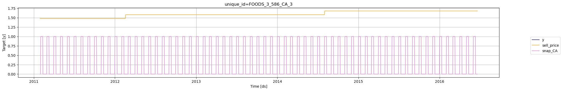
In this example, we’ll use a single time series from the M5 Competition dataset. This series represents the daily sales of a product in a Walmart store. The product-store combination that we’ll use in this notebook hasunique_id = FOODS_3_586_CA_3. This time series was chosen
because it is not intermittent and has exogenous regressors that will be
useful for forecasting.
We’ll load the following dataframes:
Y_ts: (pandas DataFrame) The target time series with columns [unique_id,ds,y].X_ts: (pandas DataFrame) Exogenous time series with columns [unique_id,ds, exogenous regressors].
statsforecast.plot method from the
StatsForecast class. This
method has multiple parameters, and the required ones to generate the
plots in this notebook are explained below.
df: A pandas dataframe with columns [unique_id,ds,y].forecasts_df: A pandas dataframe with columns [unique_id,ds] and models.engine: str =matplotlib. It can also beplotly.plotlygenerates interactive plots, whilematplotlibgenerates static plots.

sell_price: The price of the product for the given store. The price is provided per week.snap_CA: A binary variable indicating whether the store allows SNAP purchases (1 if yes, 0 otherwise). SNAP stands for Supplement Nutrition Assitance Program, and it gives individuals and families money to help them purchase food products.
Here the
unique_id is a category, but for the exogenous regressors it
needs to be a string.
plotly. We could use
statsforecast.plot, but then one of the regressors must be renamed
y, and the name must be changed back to the original before generating
the forecast.
Split train/test set
In the M5 Competition, participants had to forecast sales for the last 28 days in the dataset. We’ll use the same forecast horizon and create the train and test sets accordingly.Add exogenous regressors
The exogenous regressors need to be place after the target variabley.
Create future exogenous regressors
We need to include the future values of the exogenous regressors so that we can produce the forecasts. Notice that we already have this information inX_test.
Important If the future values of the exogenous regressors are not available, then they must be forecasted or the regressors need to be eliminated from the model. Without them, it is not possible to generate the forecast.
Train model
To generate the forecast, we’ll use AutoARIMA, which is one of the models available in StatsForecast that allows exogenous regressors. To use this model, we first need to import it fromstatsforecast.models and then we need to instantiate it. Given that
we’re working with daily data, we need to set season_length = 7.
df: The dataframe with the training data.models: The list of models defined in the previous step.freq: A string indicating the frequency of the data. See pandas’ available frequencies.n_jobs: An integer that indicates the number of jobs used in parallel processing. Use -1 to select all cores.
forecast method, which takes the following arguments.
h: An integer that represents the forecast horizon. In this case, we’ll forecast the next 28 days.X_df: A pandas dataframe with the future values of the exogenous regressors.level: A list of floats with the confidence levels of the prediction intervals. For example,level=[95]means that the range of values should include the actual future value with probability 95%.
We can plot the forecasts with the
statsforecast.plot method described
above.
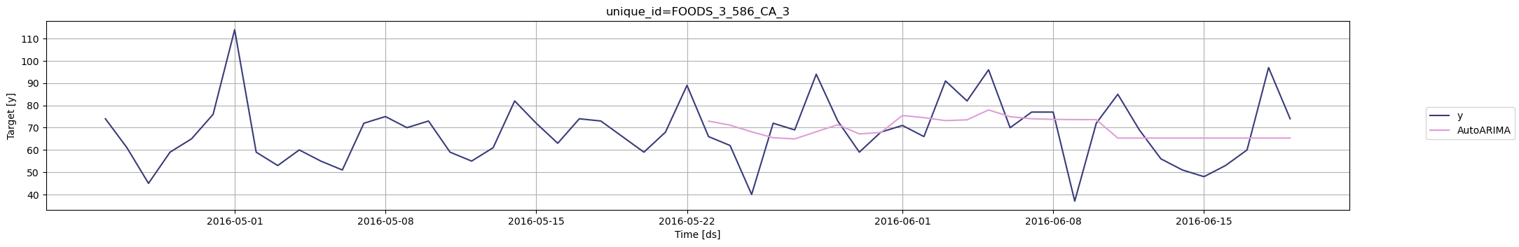
Evaluate results
We’ll merge the test set and the forecast to evaluate the accuracy using the mean absolute error (MAE).forecast method.
Notice that the data only includes unique_id, ds, and y. The
forecast method no longer requires the future values of the exogenous
regressors X_df.
sell_price and snap_CA as external
regressors helped improve the forecast.