

Minimal Example of StatsForecast
StatsForecast follows the sklearn model API. For this minimal example,
you will create an instance of the StatsForecast class and then call its
fit and predict methods. We recommend this option if speed is not
paramount and you want to explore the fitted values and parameters.
Tip
If you want to forecast many series, we recommend using the forecast
method. Check this Getting Started with multiple time
series guide.
The input to StatsForecast is always a data frame in long
format with
three columns: unique_id, ds and y:
-
The
unique_id(string, int or category) represents an identifier for the series. -
The
ds(datestamp) column should be of a format expected by Pandas, ideally YYYY-MM-DD for a date or YYYY-MM-DD HH:MM:SS for a timestamp. -
The
y(numeric) represents the measurement we wish to forecast.
| unique_id | ds | y | |
|---|---|---|---|
| 0 | AirPassengers | 1949-01-01 | 112 |
| 1 | AirPassengers | 1949-02-01 | 118 |
| 2 | AirPassengers | 1949-03-01 | 132 |
| 3 | AirPassengers | 1949-04-01 | 129 |
| 4 | AirPassengers | 1949-05-01 | 121 |
StatsForecast object with its
two required parameters: * models: a
list of models. Select the models you want from
models and import them. For this example,
we will use a AutoARIMA model. We set season_length to 12 because we
expect seasonal effects every 12 months. (See: Seasonal
periods)
freq: a string indicating the frequency of the data. (See pandas available frequencies.)
predict method takes two arguments: forecasts the next h (for
horizon) and level.
-
h(int): represents the forecast h steps into the future. In this case, 12 months ahead. -
level(list of floats): this optional parameter is used for probabilistic forecasting. Set thelevel(or confidence percentile) of your prediction interval. For example,level=[90]means that the model expects the real value to be inside that interval 90% of the times.
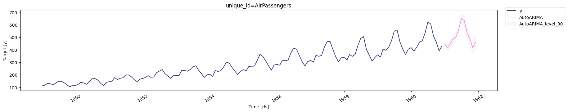
| unique_id | ds | AutoARIMA | AutoARIMA-lo-90 | AutoARIMA-hi-90 | |
|---|---|---|---|---|---|
| 7 | AirPassengers | 1961-08-01 | 633.236389 | 590.009033 | 676.463745 |
| 8 | AirPassengers | 1961-09-01 | 535.236389 | 489.558899 | 580.913940 |
| 9 | AirPassengers | 1961-10-01 | 488.236389 | 440.233795 | 536.239014 |
| 10 | AirPassengers | 1961-11-01 | 417.236389 | 367.016205 | 467.456604 |
| 11 | AirPassengers | 1961-12-01 | 459.236389 | 406.892456 | 511.580322 |
StatsForecast.plot method and
passing in your forecast dataframe.
Next Steps
- Build and end-to-end forecasting pipeline following best practices in End to End Walkthrough
- Forecast millions of series in a scalable cluster in the cloud using Spark and Nixtla
- Detect anomalies in your past observations