Cross validation

Prerequesites

This tutorial assumes basic familiarity with StatsForecast. For a minimal example visit the Quick Start

​

Introduction

Time series cross-validation is a method for evaluating how a model would have performed in the past. It works by defining a sliding window across the historical data and predicting the period following it.

Statsforecast has an implementation of time series cross-validation that is fast and easy to use. This implementation makes cross-validation a distributed operation, which makes it less time-consuming. In this notebook, we’ll use it on a subset of the M4 Competition hourly dataset.

Outline:

1. Install libraries
2. Load and explore data
3. Train model
4. Perform time series cross-validation
5. Evaluate results

Tip

You can use Colab to run this Notebook interactively

​

Install libraries

We assume that you have StatsForecast already installed. If not, check this guide for instructions on how to install StatsForecast

Install the necessary packages with pip install statsforecast

pip install statsforecast

from statsforecast import StatsForecast # required to instantiate StastForecast object and use cross-validation method

​

Load and explore the data

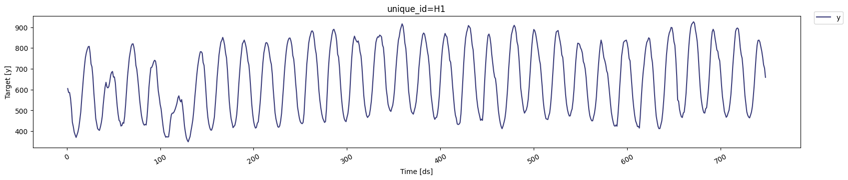
As stated in the introduction, we’ll use the M4 Competition hourly dataset. We’ll first import the data from an URL using pandas.

import pandas as pd 

Y_df = pd.read_parquet('https://datasets-nixtla.s3.amazonaws.com/m4-hourly.parquet') # load the data 
Y_df.head()

The input to StatsForecast is a data frame in long format with three columns: unique_id, ds and y:

• The unique_id (string, int, or category) represents an identifier for the series.
• The ds (datestamp or int) column should be either an integer indexing time or a datestamp in format YYYY-MM-DD or YYYY-MM-DD HH:MM:SS.
• The y (numeric) represents the measurement we wish to forecast.

The data in this example already has this format, so no changes are needed.

To keep the time required to execute this notebook to a minimum, we’ll only use one time series from the data, namely the one with unique_id == 'H1'. However, you can use as many as you want, with no additional changes to the code needed.

df = Y_df[Y_df['unique_id'] == 'H1'] # select time series

We can plot the time series we’ll work with using StatsForecast.plot method.

StatsForecast.plot(df)

​

Train model

For this example, we’ll use StastForecast AutoETS. We first need to import it from statsforecast.models and then we need to instantiate a new StatsForecast object.

The StatsForecast object has the following parameters:

• models: a list of models. Select the models you want from models and import them.
• freq: a string indicating the frequency of the data. See panda’s available frequencies.
• n_jobs: n_jobs: int, number of jobs used in the parallel processing, use -1 for all cores.

Any settings are passed into the constructor. Then you call its fit method and pass in the historical data frame df.

from statsforecast.models import AutoETS

models = [AutoETS(season_length = 24)]

sf = StatsForecast(
    df = df, 
    models = models, 
    freq = 'H', 
    n_jobs = -1
)

​

Perform time series cross-validation

Once the StatsForecastobject has been instantiated, we can use the cross_validation method, which takes the following arguments:

• df: training data frame with StatsForecast format
• h (int): represents the h steps into the future that will be forecasted
• step_size (int): step size between each window, meaning how often do you want to run the forecasting process.
• n_windows (int): number of windows used for cross-validation, meaning the number of forecasting processes in the past you want to evaluate.

For this particular example, we’ll use 3 windows of 24 hours.

crossvalidation_df = sf.cross_validation(
    df = df,
    h = 24,
    step_size = 24,
    n_windows = 3
  )

The crossvaldation_df object is a new data frame that includes the following columns:

• unique_id: index. If you dont like working with index just run crossvalidation_df.resetindex()
• ds: datestamp or temporal index
• cutoff: the last datestamp or temporal index for the n_windows.
• y: true value
• "model": columns with the model’s name and fitted value.

crossvalidation_df.head()

We’ll now plot the forecast for each cutoff period. To make the plots clearer, we’ll rename the actual values in each period.

crossvalidation_df.rename(columns = {'y' : 'actual'}, inplace = True) # rename actual values 

cutoff = crossvalidation_df['cutoff'].unique()

for k in range(len(cutoff)): 
    cv = crossvalidation_df[crossvalidation_df['cutoff'] == cutoff[k]]
    StatsForecast.plot(df, cv.loc[:, cv.columns != 'cutoff'])

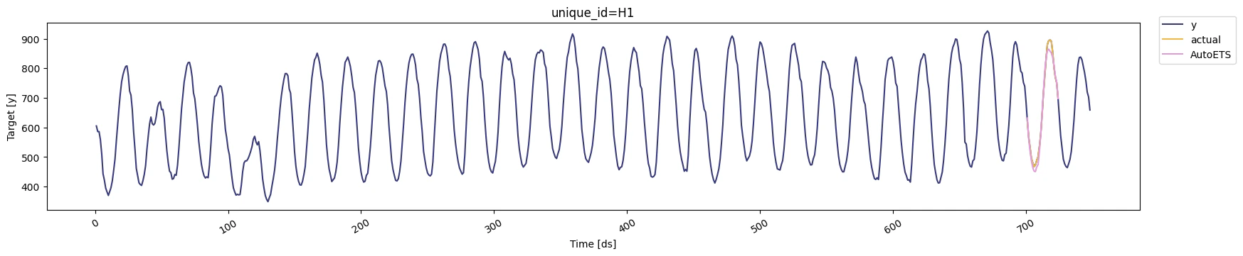
Notice that in each cutoff period, we generated a forecast for the next 24 hours using only the data y before said period.

​

Evaluate results

We can now compute the accuracy of the forecast using an appropiate accuracy metric. Here we’ll use the Root Mean Squared Error (RMSE). To do this, we first need to install datasetsforecast, a Python library developed by Nixtla that includes a function to compute the RMSE.

pip install datasetsforecast

from datasetsforecast.losses import rmse

The function to compute the RMSE takes two arguments:

1. The actual values.
2. The forecasts, in this case, AutoETS.

rmse = rmse(crossvalidation_df['actual'], crossvalidation_df['AutoETS'])
print("RMSE using cross-validation: ", rmse)

RMSE using cross-validation:  33.90342

This measure should better reflect the predictive abilities of our model, since it used different time periods to test its accuracy.

Tip

Cross validation is especially useful when comparing multiple models. Here’s an example with multiple models and time series.

​

References

Rob J. Hyndman and George Athanasopoulos (2018). “Forecasting principles and practice, Time series cross-validation”.