Interpretable Decompositions
Time series signal decomposition involves breaking down an original time series into its constituent components. By decomposing the time series, we can gain insights into underlying patterns, trends-cycles, and seasonal effects, enabling improved understanding and forecasting accuracy.
This notebook will show how to use the
NHITS
/NBEATSx
to extract these series’ components. We will:
- Installing
NeuralForecast.
- Simulate a Harmonic Signal.
- NHITS’ forecast
decomposition.
- NBEATSx’ forecast decomposition.
You can run these experiments using GPU with Google Colab.
1. Installing NeuralForecast
!pip install neuralforecast
2. Simulate a Harmonic Signal
In this example, we will consider a Harmonic signal comprising two frequencies: one low-frequency and one high-frequency.
import numpy as np
import pandas as pd
N = 10_000
T = 1.0 / 800.0 # sample spacing
x = np.linspace(0.0, N*T, N, endpoint=False)
y1 = np.sin(10.0 * 2.0*np.pi*x)
y2 = 0.5 * np.sin(100 * 2.0*np.pi*x)
y = y1 + y2
import matplotlib.pyplot as plt
plt.rcParams["axes.grid"]=True
fig, ax = plt.subplots(figsize=(6, 2.5))
plt.plot(y[-80:], label='True')
plt.plot(y1[-80:], label='Low Frequency', alpha=0.4)
plt.plot(y2[-80:], label='High Frequency', alpha=0.4)
plt.ylabel('Harmonic Signal')
plt.xlabel('Time')
plt.legend()
plt.show()
plt.close()
# Split dataset into train/test
# Last horizon observations for test
horizon = 96
Y_df = pd.DataFrame(dict(unique_id=1, ds=np.arange(len(x)), y=y))
Y_train_df = Y_df.groupby('unique_id').head(len(Y_df)-horizon).reset_index()
Y_test_df = Y_df.groupby('unique_id').tail(horizon).reset_index()
Y_test_df
index | unique_id | ds | y | |
---|---|---|---|---|
0 | 9904 | 1 | 9904 | -0.951057 |
1 | 9905 | 1 | 9905 | -0.570326 |
2 | 9906 | 1 | 9906 | -0.391007 |
3 | 9907 | 1 | 9907 | -0.499087 |
4 | 9908 | 1 | 9908 | -0.809017 |
… | … | … | … | … |
91 | 9995 | 1 | 9995 | -0.029130 |
92 | 9996 | 1 | 9996 | -0.309017 |
93 | 9997 | 1 | 9997 | -0.586999 |
94 | 9998 | 1 | 9998 | -0.656434 |
95 | 9999 | 1 | 9999 | -0.432012 |
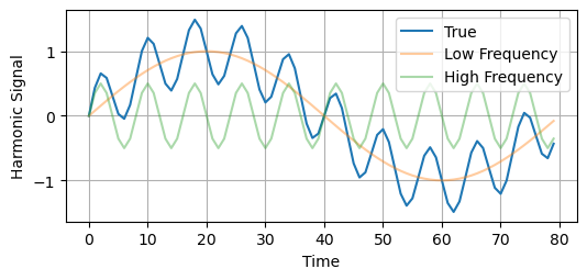
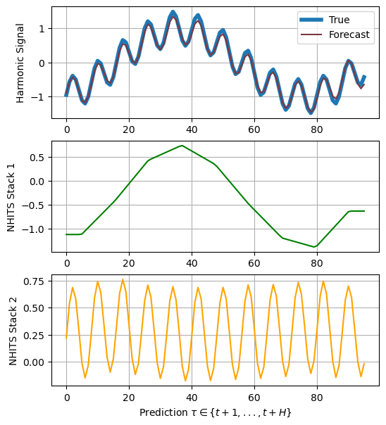
3. NHITS decomposition
We will employ
NHITS
stack-specialization to recover the latent harmonic functions.
NHITS
,
a Wavelet-inspired algorithm, allows for breaking down a time series
into various scales or resolutions, aiding in the identification of
localized patterns or features. The expressivity ratios for each layer
enable control over the model’s stack specialization.
from neuralforecast.models import NHITS, NBEATSx
from neuralforecast import NeuralForecast
from neuralforecast.losses.pytorch import HuberLoss, MQLoss
models = [NHITS(h=horizon, # Forecast horizon
input_size=2 * horizon, # Length of input sequence
loss=HuberLoss(), # Robust Huber Loss
max_steps=1000, # Number of steps to train
dropout_prob_theta=0.5,
interpolation_mode='linear',
stack_types=['identity']*2,
n_blocks=[1, 1],
mlp_units=[[64, 64],[64, 64]],
n_freq_downsample=[10, 1], # Inverse expressivity ratios for NHITS' stacks specialization
val_check_steps=10, # Frequency of validation signal (affects early stopping)
)
]
nf = NeuralForecast(models=models, freq='M')
nf.fit(df=Y_train_df)
Global seed set to 1
from neuralforecast.tsdataset import TimeSeriesDataset
# NHITS decomposition plot
model = nf.models[0]
dataset, *_ = TimeSeriesDataset.from_df(df = Y_train_df)
y_hat = model.decompose(dataset=dataset)
Predicting DataLoader 0: 100%|██████████| 1/1 [00:00<00:00, 20.68it/s]
fig, ax = plt.subplots(3, 1, figsize=(6, 7))
ax[0].plot(Y_test_df['y'].values, label='True', linewidth=4)
ax[0].plot(y_hat.sum(axis=1).flatten(), label='Forecast', color="#7B3841")
ax[0].legend()
ax[0].set_ylabel('Harmonic Signal')
ax[1].plot(y_hat[0,1]+y_hat[0,0], label='stack1', color="green")
ax[1].set_ylabel('NHITS Stack 1')
ax[2].plot(y_hat[0,2], label='stack2', color="orange")
ax[2].set_ylabel('NHITS Stack 2')
ax[2].set_xlabel(r'Prediction $\tau \in \{t+1,..., t+H\}$')
plt.show()
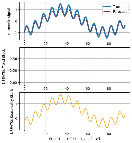
4. NBEATSx decomposition
Here we will employ
NBEATSx
interpretable basis projection to recover the latent harmonic functions.
NBEATSx
,
this network in its interpretable variant sequentially projects the
signal into polynomials and harmonic basis to learn trend and
seasonality components:
In contrast to
NHITS
’
wavelet-like projections the basis heavily determine the behavior of the
projections. And the Fourier projections are not capable of being
immediately decomposed into individual frequencies.
models = [NBEATSx(h=horizon, # Forecast horizon
input_size=2 * horizon, # Length of input sequence
loss=HuberLoss(), # Robust Huber Loss
max_steps=1000, # Number of steps to train
dropout_prob_theta=0.5,
stack_types=['trend', 'seasonality'], # Harmonic/Trend projection basis
n_polynomials=0, # Lower frequencies can be captured by polynomials
n_blocks=[1, 1],
mlp_units=[[64, 64],[64, 64]],
val_check_steps=10, # Frequency of validation signal (affects early stopping)
)
]
nf = NeuralForecast(models=models, freq='M')
nf.fit(df=Y_train_df)
Global seed set to 1
# NBEATSx decomposition plot
model = nf.models[0]
dataset, *_ = TimeSeriesDataset.from_df(df = Y_train_df)
y_hat = model.decompose(dataset=dataset)
Predicting DataLoader 0: 100%|██████████| 1/1 [00:00<00:00, 112.51it/s]
fig, ax = plt.subplots(3, 1, figsize=(6, 7))
ax[0].plot(Y_test_df['y'].values, label='True', linewidth=4)
ax[0].plot(y_hat.sum(axis=1).flatten(), label='Forecast', color="#7B3841")
ax[0].legend()
ax[0].set_ylabel('Harmonic Signal')
ax[1].plot(y_hat[0,1]+y_hat[0,0], label='stack1', color="green")
ax[1].set_ylabel('NBEATSx Trend Stack')
ax[2].plot(y_hat[0,2], label='stack2', color="orange")
ax[2].set_ylabel('NBEATSx Seasonality Stack')
ax[2].set_xlabel(r'Prediction $\tau \in \{t+1,..., t+H\}$')
plt.show()
References
- Cristian Challu, Kin G. Olivares, Boris N. Oreshkin, Federico
Garza, Max Mergenthaler-Canseco, Artur Dubrawski (2023). NHITS:
Neural Hierarchical Interpolation for Time Series
Forecasting.
- Boris N. Oreshkin, Dmitri Carpov, Nicolas Chapados, Yoshua Bengio
(2019). “N-BEATS: Neural basis expansion analysis for interpretable
time series forecasting”.
- Kin G. Olivares, Cristian Challu, Grzegorz Marcjasz, Rafał Weron, Artur Dubrawski (2021). “Neural basis expansion analysis with exogenous variables: Forecasting electricity prices with NBEATSx”.