

| unique_id | ds | y | |
|---|---|---|---|
| 86796 | H196 | 1 | 11.8 |
| 86797 | H196 | 2 | 11.4 |
| 86798 | H196 | 3 | 11.1 |
| 86799 | H196 | 4 | 10.8 |
| 86800 | H196 | 5 | 10.6 |
| … | … | … | … |
| 325235 | H413 | 1004 | 99.0 |
| 325236 | H413 | 1005 | 88.0 |
| 325237 | H413 | 1006 | 47.0 |
| 325238 | H413 | 1007 | 41.0 |
| 325239 | H413 | 1008 | 34.0 |
Creating the forecaster
Fitting and predicting
| unique_id | ds | LGBMRegressor | |
|---|---|---|---|
| 0 | H196 | 961 | 16.079737 |
| 1 | H196 | 962 | 15.679737 |
| 2 | H196 | 963 | 15.279737 |
| 3 | H196 | 964 | 14.979737 |
| 4 | H196 | 965 | 14.679737 |
| 5 | H256 | 961 | 13.279737 |
| 6 | H256 | 962 | 12.679737 |
| 7 | H256 | 963 | 12.379737 |
| 8 | H256 | 964 | 12.079737 |
| 9 | H256 | 965 | 11.879737 |
| 10 | H381 | 961 | 56.939977 |
| 11 | H381 | 962 | 40.314608 |
| 12 | H381 | 963 | 33.859013 |
| 13 | H381 | 964 | 15.498139 |
| 14 | H381 | 965 | 25.722674 |
| 15 | H413 | 961 | 25.131194 |
| 16 | H413 | 962 | 19.177421 |
| 17 | H413 | 963 | 21.250829 |
| 18 | H413 | 964 | 18.743132 |
| 19 | H413 | 965 | 16.027263 |
| unique_id | ds | cutoff | y | LGBMRegressor | |
|---|---|---|---|---|---|
| 0 | H196 | 951 | 950 | 24.4 | 24.288850 |
| 1 | H196 | 952 | 950 | 24.3 | 24.188850 |
| 2 | H196 | 953 | 950 | 23.8 | 23.688850 |
| 3 | H196 | 954 | 950 | 22.8 | 22.688850 |
| 4 | H196 | 955 | 950 | 21.2 | 21.088850 |
| 5 | H256 | 951 | 950 | 19.5 | 19.688850 |
| 6 | H256 | 952 | 950 | 19.4 | 19.488850 |
| 7 | H256 | 953 | 950 | 18.9 | 19.088850 |
| 8 | H256 | 954 | 950 | 18.3 | 18.388850 |
| 9 | H256 | 955 | 950 | 17.0 | 17.088850 |
| 10 | H381 | 951 | 950 | 182.0 | 208.327270 |
| 11 | H381 | 952 | 950 | 222.0 | 247.768326 |
| 12 | H381 | 953 | 950 | 288.0 | 277.965997 |
| 13 | H381 | 954 | 950 | 264.0 | 321.532857 |
| 14 | H381 | 955 | 950 | 191.0 | 206.316903 |
| 15 | H413 | 951 | 950 | 77.0 | 60.972692 |
| 16 | H413 | 952 | 950 | 91.0 | 54.936494 |
| 17 | H413 | 953 | 950 | 76.0 | 73.949203 |
| 18 | H413 | 954 | 950 | 68.0 | 67.087417 |
| 19 | H413 | 955 | 950 | 68.0 | 75.896022 |
| 20 | H196 | 956 | 955 | 19.3 | 19.287891 |
| 21 | H196 | 957 | 955 | 18.2 | 18.187891 |
| 22 | H196 | 958 | 955 | 17.5 | 17.487891 |
| 23 | H196 | 959 | 955 | 16.9 | 16.887891 |
| 24 | H196 | 960 | 955 | 16.5 | 16.487891 |
| 25 | H256 | 956 | 955 | 15.5 | 15.687891 |
| 26 | H256 | 957 | 955 | 14.7 | 14.787891 |
| 27 | H256 | 958 | 955 | 14.1 | 14.287891 |
| 28 | H256 | 959 | 955 | 13.6 | 13.787891 |
| 29 | H256 | 960 | 955 | 13.2 | 13.387891 |
| 30 | H381 | 956 | 955 | 130.0 | 124.117828 |
| 31 | H381 | 957 | 955 | 113.0 | 119.180350 |
| 32 | H381 | 958 | 955 | 94.0 | 105.356552 |
| 33 | H381 | 959 | 955 | 192.0 | 127.095338 |
| 34 | H381 | 960 | 955 | 87.0 | 119.875754 |
| 35 | H413 | 956 | 955 | 59.0 | 67.993133 |
| 36 | H413 | 957 | 955 | 58.0 | 69.869815 |
| 37 | H413 | 958 | 955 | 53.0 | 34.717960 |
| 38 | H413 | 959 | 955 | 38.0 | 47.665581 |
| 39 | H413 | 960 | 955 | 46.0 | 45.940137 |
| unique_id | ds | |
|---|---|---|
| 0 | H196 | 961 |
| 1 | H256 | 961 |
| 2 | H381 | 961 |
| 3 | H413 | 961 |
| unique_id | ds | y | LGBMRegressor | |
|---|---|---|---|---|
| 0 | H196 | 193 | 12.7 | 12.671271 |
| 1 | H196 | 194 | 12.3 | 12.271271 |
| 2 | H196 | 195 | 11.9 | 11.871271 |
| 3 | H196 | 196 | 11.7 | 11.671271 |
| 4 | H196 | 197 | 11.4 | 11.471271 |
| … | … | … | … | … |
| 3067 | H413 | 956 | 59.0 | 68.280574 |
| 3068 | H413 | 957 | 58.0 | 70.427570 |
| 3069 | H413 | 958 | 53.0 | 44.767965 |
| 3070 | H413 | 959 | 38.0 | 48.691257 |
| 3071 | H413 | 960 | 46.0 | 46.652238 |
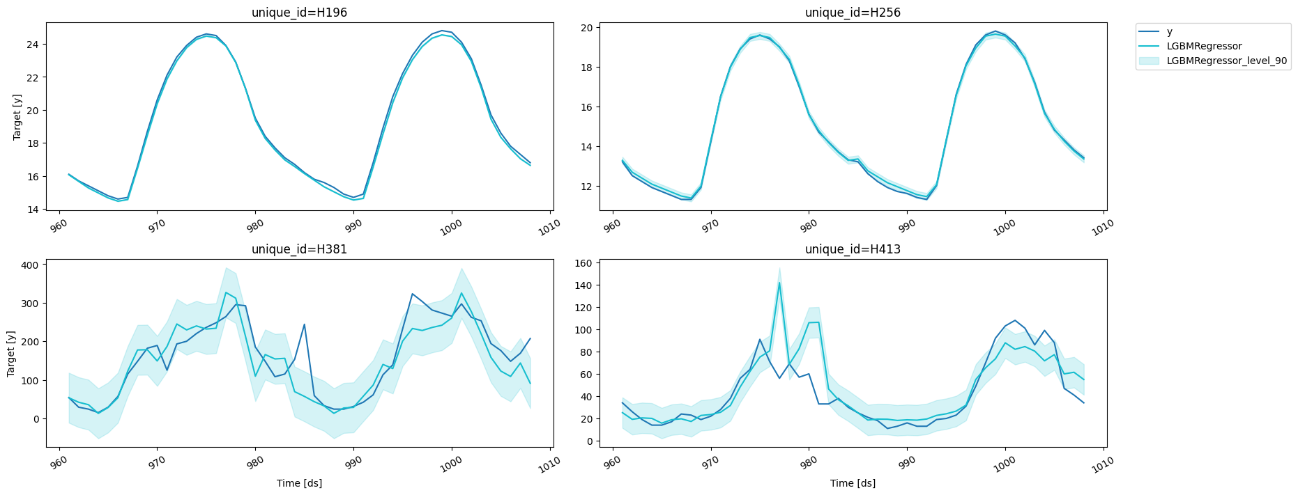
| unique_id | ds | y | LGBMRegressor | LGBMRegressor-lo-90 | LGBMRegressor-hi-90 | |
|---|---|---|---|---|---|---|
| 0 | H196 | 193 | 12.7 | 12.671271 | 12.540634 | 12.801909 |
| 1 | H196 | 194 | 12.3 | 12.271271 | 12.140634 | 12.401909 |
| 2 | H196 | 195 | 11.9 | 11.871271 | 11.740634 | 12.001909 |
| 3 | H196 | 196 | 11.7 | 11.671271 | 11.540634 | 11.801909 |
| 4 | H196 | 197 | 11.4 | 11.471271 | 11.340634 | 11.601909 |
| … | … | … | … | … | … | … |
| 3067 | H413 | 956 | 59.0 | 68.280574 | 58.846640 | 77.714509 |
| 3068 | H413 | 957 | 58.0 | 70.427570 | 60.993636 | 79.861504 |
| 3069 | H413 | 958 | 53.0 | 44.767965 | 35.334031 | 54.201899 |
| 3070 | H413 | 959 | 38.0 | 48.691257 | 39.257323 | 58.125191 |
| 3071 | H413 | 960 | 46.0 | 46.652238 | 37.218304 | 56.086172 |

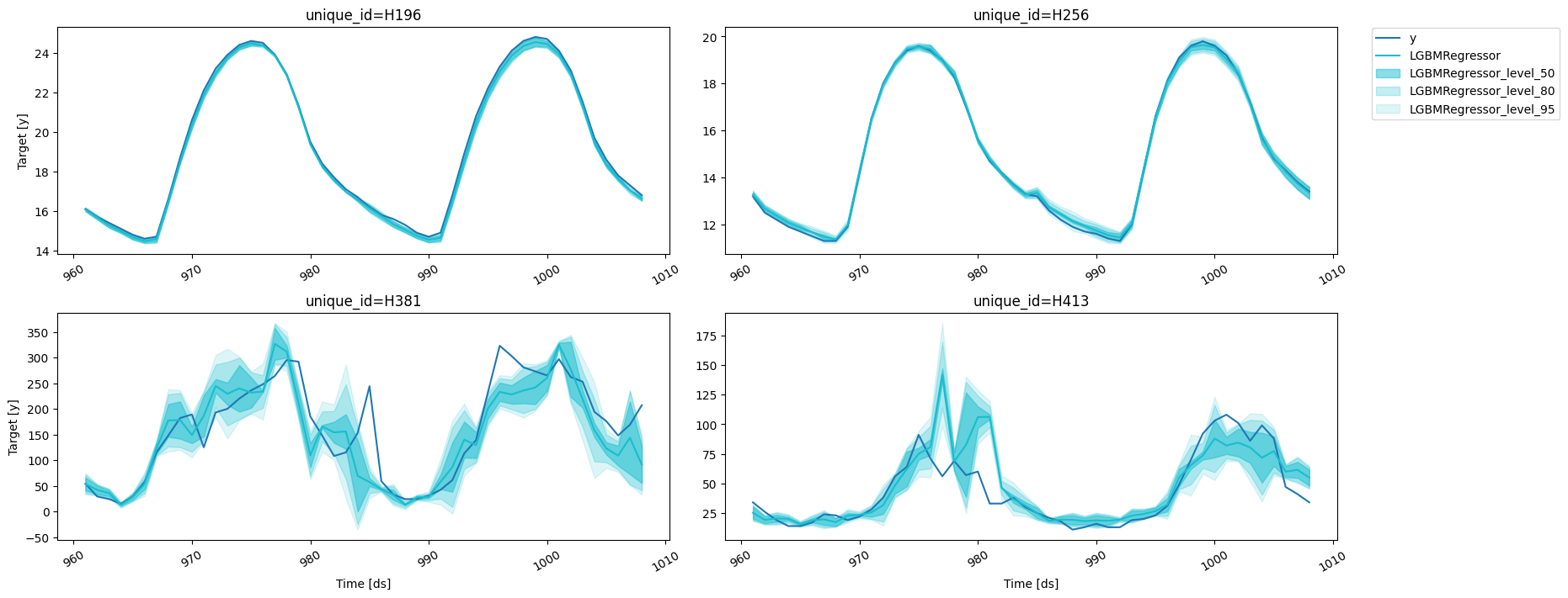
Prediction intervals
WithMLForecast,
you can generate prediction intervals using Conformal Prediction. To
configure Conformal Prediction, you need to pass an instance of the
PredictionIntervals
class to the prediction_intervals argument of the fit method. The
class takes three parameters: n_windows, h and method.
n_windowsrepresents the number of cross-validation windows used to calibrate the intervalshis the forecast horizonmethodcan beconformal_distributionorconformal_error;conformal_distribution(default) creates forecasts paths based on the cross-validation errors and calculate quantiles using those paths, on the other handconformal_errorcalculates the error quantiles to produce prediction intervals. The strategy will adjust the intervals for each horizon step, resulting in different widths for each step. Please note that a minimum of 2 cross-validation windows must be used.
predict method using the level argument. Levels must lie between
0 and 100.
| unique_id | ds | LGBMRegressor | LGBMRegressor-lo-95 | LGBMRegressor-lo-80 | LGBMRegressor-lo-50 | LGBMRegressor-hi-50 | LGBMRegressor-hi-80 | LGBMRegressor-hi-95 | |
|---|---|---|---|---|---|---|---|---|---|
| 0 | H196 | 961 | 16.071271 | 15.958042 | 15.971271 | 16.005091 | 16.137452 | 16.171271 | 16.184501 |
| 1 | H196 | 962 | 15.671271 | 15.553632 | 15.553632 | 15.578632 | 15.763911 | 15.788911 | 15.788911 |
| 2 | H196 | 963 | 15.271271 | 15.153632 | 15.153632 | 15.162452 | 15.380091 | 15.388911 | 15.388911 |
| 3 | H196 | 964 | 14.971271 | 14.858042 | 14.871271 | 14.905091 | 15.037452 | 15.071271 | 15.084501 |
| 4 | H196 | 965 | 14.671271 | 14.553632 | 14.553632 | 14.562452 | 14.780091 | 14.788911 | 14.788911 |
h=1 to the
PredictionIntervals
class. The caveat of this strategy is that in some cases, variance of
the absolute residuals maybe be small (even zero), so the intervals may
be too narrow.
Forecast using a pretrained model
MLForecast allows you to use a pretrained model to generate forecasts for a new dataset. Simply provide a pandas dataframe containing the new observations as the value for thenew_df argument when calling the
predict method. The dataframe should have the same structure as the
one used to fit the model, including any features and time series data.
The function will then use the pretrained model to generate forecasts
for the new observations. This allows you to easily apply a pretrained
model to a new dataset and generate forecasts without the need to
retrain the model.

Preprocess
If you want to take a look at the data that will be used to train the models you can callForecast.preprocess.
| unique_id | ds | y | lag24 | lag48 | lag72 | lag96 | lag120 | lag144 | lag168 | exponentially_weighted_mean_lag48_alpha0.3 | |
|---|---|---|---|---|---|---|---|---|---|---|---|
| 86988 | H196 | 193 | 0.1 | 0.0 | 0.0 | 0.0 | 0.3 | 0.1 | 0.1 | 0.3 | 0.002810 |
| 86989 | H196 | 194 | 0.1 | -0.1 | 0.1 | 0.0 | 0.3 | 0.1 | 0.1 | 0.3 | 0.031967 |
| 86990 | H196 | 195 | 0.1 | -0.1 | 0.1 | 0.0 | 0.3 | 0.1 | 0.2 | 0.1 | 0.052377 |
| 86991 | H196 | 196 | 0.1 | 0.0 | 0.0 | 0.0 | 0.3 | 0.2 | 0.1 | 0.2 | 0.036664 |
| 86992 | H196 | 197 | 0.0 | 0.0 | 0.0 | 0.1 | 0.2 | 0.2 | 0.1 | 0.2 | 0.025665 |
| … | … | … | … | … | … | … | … | … | … | … | … |
| 325187 | H413 | 956 | 0.0 | 10.0 | 1.0 | 6.0 | -53.0 | 44.0 | -21.0 | 21.0 | 7.963225 |
| 325188 | H413 | 957 | 9.0 | 10.0 | 10.0 | -7.0 | -46.0 | 27.0 | -19.0 | 24.0 | 8.574257 |
| 325189 | H413 | 958 | 16.0 | 8.0 | 5.0 | -9.0 | -36.0 | 32.0 | -13.0 | 8.0 | 7.501980 |
| 325190 | H413 | 959 | -3.0 | 17.0 | -7.0 | 2.0 | -31.0 | 22.0 | 5.0 | -2.0 | 3.151386 |
| 325191 | H413 | 960 | 15.0 | 11.0 | -6.0 | -5.0 | -17.0 | 22.0 | -18.0 | 10.0 | 0.405970 |
Forecast.fit_models, since this
only stores the series information.
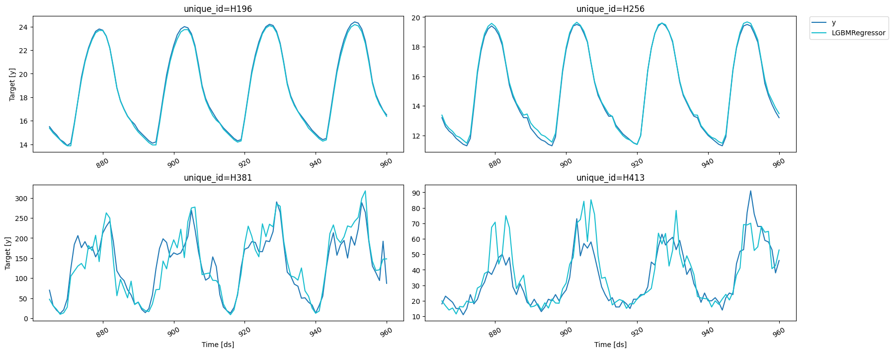
MLForecast.cross_validation,
which takes our data and performs the process described above for
n_windows times where each window has h validation samples in it.
For example, if we have 100 samples and we want to perform 2 backtests
each of size 14, the splits will be as follows:
- Train: 1 to 72. Validation: 73 to 86.
- Train: 1 to 86. Validation: 87 to 100.
step_size argument. For example, if we have 100 samples and we want to
perform 2 backtests each of size 14 and move one step ahead in each fold
(step_size=1), the splits will be as follows:
- Train: 1 to 85. Validation: 86 to 99.
- Train: 1 to 86. Validation: 87 to 100.
refit=False. This allows you to evaluate the
performance of your models using multiple window sizes without having to
retrain them each time.
| unique_id | ds | cutoff | y | LGBMRegressor | |
|---|---|---|---|---|---|
| 0 | H196 | 865 | 864 | 15.5 | 15.373393 |
| 1 | H196 | 866 | 864 | 15.1 | 14.973393 |
| 2 | H196 | 867 | 864 | 14.8 | 14.673393 |
| 3 | H196 | 868 | 864 | 14.4 | 14.373393 |
| 4 | H196 | 869 | 864 | 14.2 | 14.073393 |
| … | … | … | … | … | … |
| 379 | H413 | 956 | 912 | 59.0 | 64.284167 |
| 380 | H413 | 957 | 912 | 58.0 | 64.830429 |
| 381 | H413 | 958 | 912 | 53.0 | 40.726851 |
| 382 | H413 | 959 | 912 | 38.0 | 42.739657 |
| 383 | H413 | 960 | 912 | 46.0 | 52.802769 |
fitted=True we can access the predictions for the
training sets as well with the cross_validation_fitted_values method.
| unique_id | ds | fold | y | LGBMRegressor | |
|---|---|---|---|---|---|
| 0 | H196 | 193 | 0 | 12.7 | 12.673393 |
| 1 | H196 | 194 | 0 | 12.3 | 12.273393 |
| 2 | H196 | 195 | 0 | 11.9 | 11.873393 |
| 3 | H196 | 196 | 0 | 11.7 | 11.673393 |
| 4 | H196 | 197 | 0 | 11.4 | 11.473393 |
| … | … | … | … | … | … |
| 5563 | H413 | 908 | 1 | 49.0 | 50.620196 |
| 5564 | H413 | 909 | 1 | 39.0 | 35.972331 |
| 5565 | H413 | 910 | 1 | 29.0 | 29.359678 |
| 5566 | H413 | 911 | 1 | 24.0 | 25.784563 |
| 5567 | H413 | 912 | 1 | 20.0 | 23.168413 |
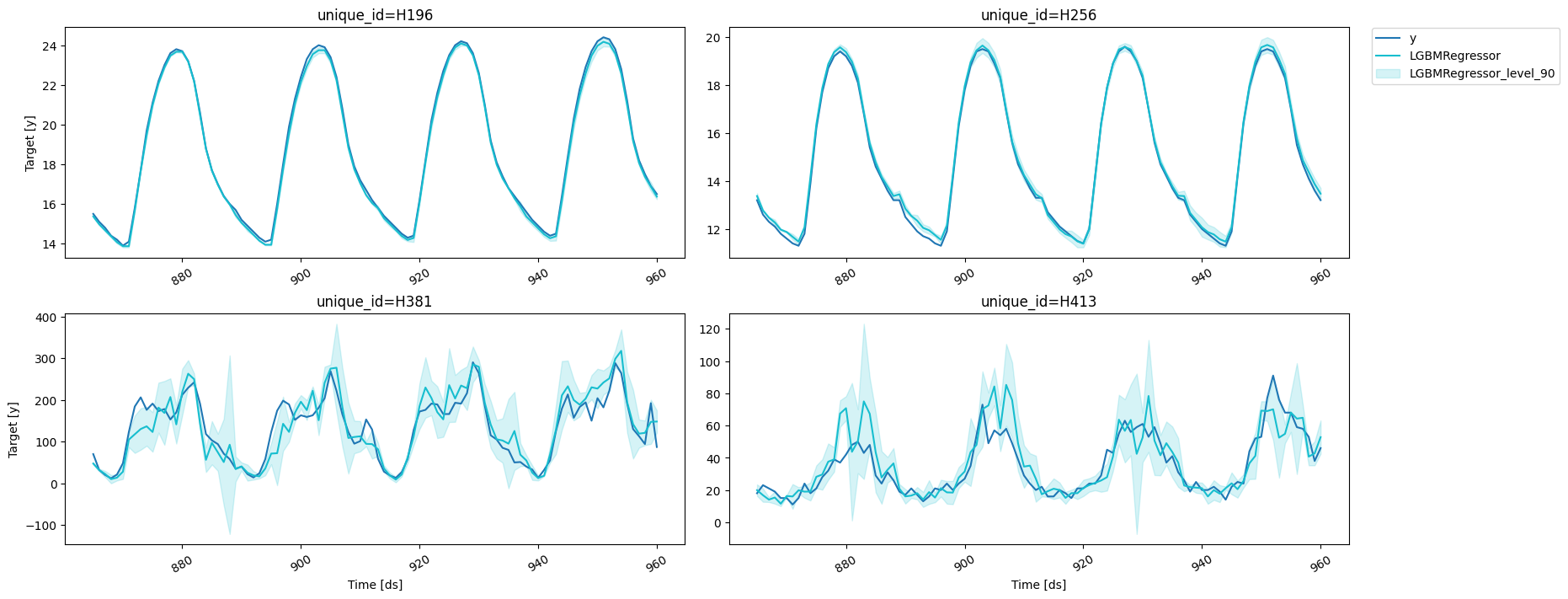
prediction_intervals as well as values for the width through levels.
| unique_id | ds | cutoff | y | LGBMRegressor | LGBMRegressor-lo-90 | LGBMRegressor-lo-80 | LGBMRegressor-hi-80 | LGBMRegressor-hi-90 | |
|---|---|---|---|---|---|---|---|---|---|
| 0 | H196 | 865 | 864 | 15.5 | 15.373393 | 15.311379 | 15.316528 | 15.430258 | 15.435407 |
| 1 | H196 | 866 | 864 | 15.1 | 14.973393 | 14.940556 | 14.940556 | 15.006230 | 15.006230 |
| 2 | H196 | 867 | 864 | 14.8 | 14.673393 | 14.606230 | 14.606230 | 14.740556 | 14.740556 |
| 3 | H196 | 868 | 864 | 14.4 | 14.373393 | 14.306230 | 14.306230 | 14.440556 | 14.440556 |
| 4 | H196 | 869 | 864 | 14.2 | 14.073393 | 14.006230 | 14.006230 | 14.140556 | 14.140556 |
| … | … | … | … | … | … | … | … | … | … |
| 379 | H413 | 956 | 912 | 59.0 | 64.284167 | 29.890099 | 34.371545 | 94.196788 | 98.678234 |
| 380 | H413 | 957 | 912 | 58.0 | 64.830429 | 56.874572 | 57.827689 | 71.833169 | 72.786285 |
| 381 | H413 | 958 | 912 | 53.0 | 40.726851 | 35.296195 | 35.846206 | 45.607495 | 46.157506 |
| 382 | H413 | 959 | 912 | 38.0 | 42.739657 | 35.292153 | 35.807640 | 49.671674 | 50.187161 |
| 383 | H413 | 960 | 912 | 46.0 | 52.802769 | 42.465597 | 43.895670 | 61.709869 | 63.139941 |
refit argument allows us to control if we want to retrain the
models in every window. It can either be:
- A boolean: True will retrain on every window and False only on the first one.
- A positive integer: The models will be trained on the first window
and then every
refitwindows.
Using LightGBMCV to tune your forecasts
Once you’ve found a set of features and parameters that work for your problem you can build a forecast object from it usingMLForecast.from_cv,
which takes the trained
LightGBMCV
object and builds an
MLForecast
object that will use the same features and parameters. Then you can call
fit and predict as you normally would.