Quick start (local)

​

Main concepts

The main component of mlforecast is the MLForecast class, which abstracts away:

• Feature engineering and model training through MLForecast.fit
• Feature updates and multi step ahead predictions through MLForecast.predict

​

Data format

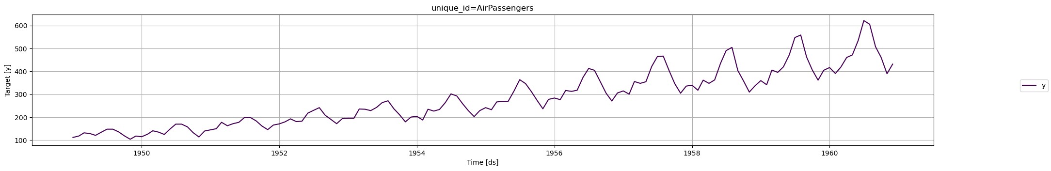
The data is expected to be a pandas dataframe in long format, that is, each row represents an observation of a single serie at a given time, with at least three columns:

• id_col: column that identifies each serie.
• target_col: column that has the series values at each timestamp.
• time_col: column that contains the time the series value was observed. These are usually timestamps, but can also be consecutive integers.

Here we present an example using the classic Box & Jenkins airline data, which measures monthly totals of international airline passengers from 1949 to 1960. Source: Box, G. E. P., Jenkins, G. M. and Reinsel, G. C. (1976) Time Series Analysis, Forecasting and Control. Third Edition. Holden-Day. Series G.

import pandas as pd
from utilsforecast.plotting import plot_series

df = pd.read_csv('https://datasets-nixtla.s3.amazonaws.com/air-passengers.csv', parse_dates=['ds'])
df.head()

df['unique_id'].value_counts()

AirPassengers    144
Name: unique_id, dtype: int64

Here the unique_id column has the same value for all rows because this is a single time series, you can have multiple time series by stacking them together and having a column that differentiates them.

We also have the ds column that contains the timestamps, in this case with a monthly frequency, and the y column that contains the series values in each timestamp.

​

Modeling

fig = plot_series(df)

We can see that the serie has a clear trend, so we can take the first difference, i.e. take each value and subtract the value at the previous month. This can be achieved by passing an mlforecast.target_transforms.Differences([1]) instance to target_transforms.

We can then train a linear regression using the value from the same month at the previous year (lag 12) as a feature, this is done by passing lags=[12].

from mlforecast import MLForecast
from mlforecast.target_transforms import Differences
from sklearn.linear_model import LinearRegression

fcst = MLForecast(
    models=LinearRegression(),
    freq='MS',  # our serie has a monthly frequency
    lags=[12],
    target_transforms=[Differences([1])],
)
fcst.fit(df)

MLForecast(models=[LinearRegression], freq=MS, lag_features=['lag12'], date_features=[], num_threads=1)

The previous line computed the features and trained the model, so now we’re ready to compute our forecasts.

​

Forecasting

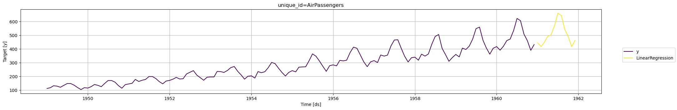
Compute the forecast for the next 12 months

preds = fcst.predict(12)
preds

​

Visualize results

We can visualize what our prediction looks like.

fig = plot_series(df, preds)

And that’s it! You’ve trained a linear regression to predict the air passengers for 1961.