Access and interpret the models after fitting
Data setup
| unique_id | ds | y | |
|---|---|---|---|
| 0 | id_0 | 2000-01-01 | 0.322947 |
| 1 | id_0 | 2000-01-02 | 1.218794 |
| 2 | id_0 | 2000-01-03 | 2.445887 |
| 3 | id_0 | 2000-01-04 | 3.481831 |
| 4 | id_0 | 2000-01-05 | 4.191721 |
Training
Suppose that you want to train a linear regression model using the day of the week and lag1 as features.MLForecast.fit does is save the required data for the predict
step and also train the models (in this case the linear regression). The
trained models are available in the MLForecast.models_ attribute,
which is a dictionary where the keys are the model names and the values
are the model themselves.
Inspect parameters
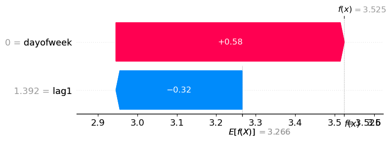
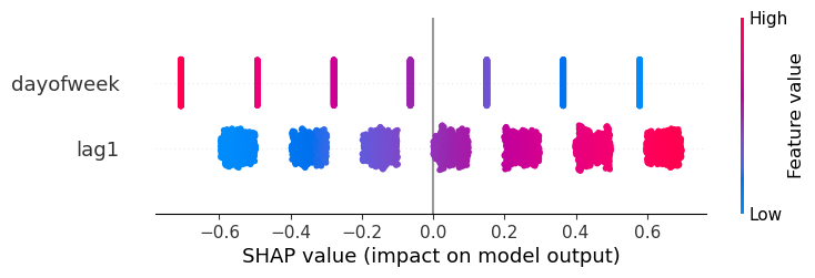
We can access the linear regression coefficients in the following way:SHAP
Training set
If you need to generate the training data you can useMLForecast.preprocess.
| unique_id | ds | y | lag1 | dayofweek | |
|---|---|---|---|---|---|
| 1 | id_0 | 2000-01-02 | 1.218794 | 0.322947 | 6 |
| 2 | id_0 | 2000-01-03 | 2.445887 | 1.218794 | 0 |
| 3 | id_0 | 2000-01-04 | 3.481831 | 2.445887 | 1 |
| 4 | id_0 | 2000-01-05 | 4.191721 | 3.481831 | 2 |
| 5 | id_0 | 2000-01-06 | 5.395863 | 4.191721 | 3 |
| lag1 | dayofweek | |
|---|---|---|
| 1 | 0.322947 | 6 |
| 2 | 1.218794 | 0 |
| 3 | 2.445887 | 1 |
| 4 | 3.481831 | 2 |
| 5 | 4.191721 | 3 |
Predictions
Sometimes you want to determine why the model gave a specific prediction. In order to do this you need the input features, which aren’t returned by default, but you can retrieve them using a callback.| unique_id | ds | lr | |
|---|---|---|---|
| 0 | id_0 | 2000-08-10 | 3.468643 |
| 1 | id_1 | 2000-04-07 | 3.016877 |
| 2 | id_2 | 2000-06-16 | 2.815249 |
| 3 | id_3 | 2000-08-30 | 4.048894 |
| 4 | id_4 | 2001-01-08 | 3.524532 |
SaveFeatures.get_features
| lag1 | dayofweek | |
|---|---|---|
| 0 | 4.343744 | 3 |
| 1 | 3.150799 | 4 |
| 2 | 2.137412 | 4 |
| 3 | 6.182456 | 2 |
| 4 | 1.391698 | 0 |
'id_4'.