

detect_anomalies_online method. You
will learn how to quickly start using this new endpoint and understand
its key differences from the historical anomaly detection endpoint. New
features include: * More flexibility and control over the anomaly
detection process * Perform univariate and multivariate anomaly
detection * Detect anomalies on stream data
👍 Use an Azure AI endpoint To use an Azure AI endpoint, set thebase_urlargument:nixtla_client = NixtlaClient(base_url="you azure ai endpoint", api_key="your api_key")
1. Dataset
In this notebook, we use a minute-level time series dataset that monitors server usage. This is a good example of a streaming data scenario, as the task is to detect server failures or downtime.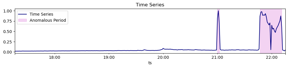
2. Detect anomalies in real time
Thedetect_anomalies_online method detect anomalies in a time series
leveraging TimeGPT’s forecast power. It uses the forecast error in
deciding the anomalous step so you can specify and tune the parameters
like that of the forecast method. This function will return a
dataframe that contains anomaly flags and anomaly score (its absolute
value quantifies the abnormality of the value).
To perfom real-time anomaly detection, set the following parameters:
df: A pandas DataFrame containing the time series data.time_col: The column that identifies the datestamp.target_col: The variable to forecast.h: Horizon is the number of steps ahead to make forecast.freq: The frequency of the time series in Pandas format.level: Percentile of scores distribution at which the threshold is set, controlling how strictly anomalies are flagged. Default at 99%.detection_size: The number of steps to analyze for anomaly at the end of time series.
| unique_id | ts | y | TimeGPT | anomaly | anomaly_score | TimeGPT-hi-99 | TimeGPT-lo-99 | |
|---|---|---|---|---|---|---|---|---|
| 95 | machine-1-1_y_29 | 2020-02-01 22:11:00 | 0.606017 | 0.544625 | True | 18.463266 | 0.553161 | 0.536090 |
| 96 | machine-1-1_y_29 | 2020-02-01 22:12:00 | 0.044413 | 0.570869 | True | -158.933850 | 0.579404 | 0.562333 |
| 97 | machine-1-1_y_29 | 2020-02-01 22:13:00 | 0.038682 | 0.560303 | True | -157.474880 | 0.568839 | 0.551767 |
| 98 | machine-1-1_y_29 | 2020-02-01 22:14:00 | 0.024355 | 0.521797 | True | -150.178240 | 0.530333 | 0.513261 |
| 99 | machine-1-1_y_29 | 2020-02-01 22:15:00 | 0.044413 | 0.467860 | True | -127.848560 | 0.476396 | 0.459325 |
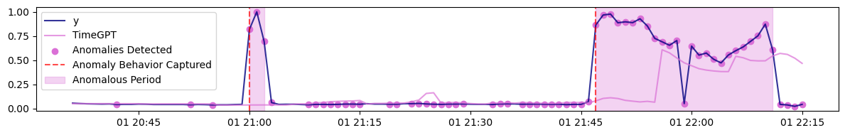
📘 In this example, we use a detection size of 100 to illustrate the anomaly detection process. In practice, using a smaller detection size and running the detection more frequently improves granularity and enables more timely identification of anomalies as they occur.From the plot, we observe that both anomalous periods were detected right as they arose. For further methods on improving detection accuracy and customizing anomaly detection, read our other tutorials on online anomaly detection.
detect_anomalies_online method, refer
to the tutorial (coming soon).