

- MAE of TimeGPT is 18.6% better than N-HiTS
- sMAPE of TimeGPT is 31.1% better than N-HiTS
- TimeGPT generated predictions in 4.3 seconds, which is 90% faster than training and predicting with N-HiTS.
Initial setup
First, we load the required packages for this experiment.NixtlaClient
to use TimeGPT.
👍 Use an Azure AI endpoint To use an Azure AI endpoint, remember to set also thebase_urlargument:nixtla_client = NixtlaClient(base_url="you azure ai endpoint", api_key="your api_key")
Read the data
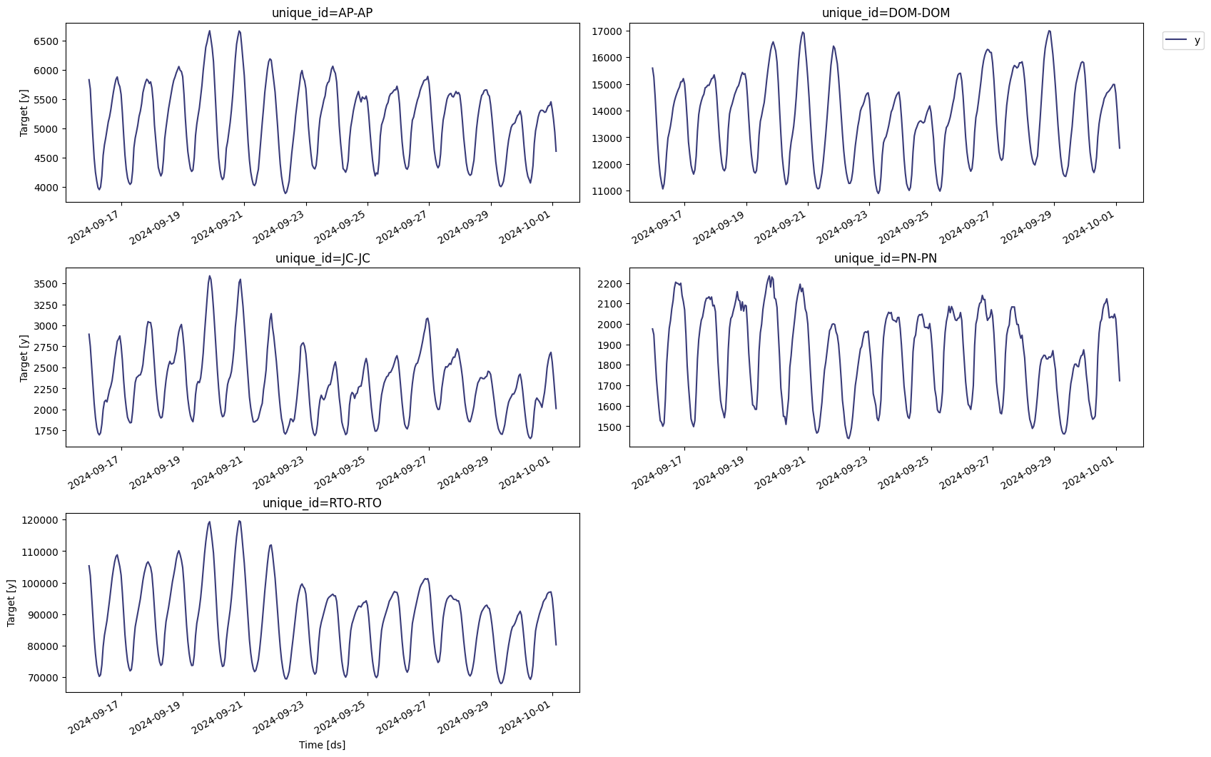
Here, we load in the inbound energy transmission time series.| unique_id | ds | y | |
|---|---|---|---|
| 0 | AP-AP | 2023-10-01 04:00:00+00:00 | 4042.513 |
| 1 | AP-AP | 2023-10-01 05:00:00+00:00 | 3850.067 |
| 8784 | DOM-DOM | 2023-10-01 04:00:00+00:00 | 10732.435 |
| 8785 | DOM-DOM | 2023-10-01 05:00:00+00:00 | 10314.211 |
| 17568 | JC-JC | 2023-10-01 04:00:00+00:00 | 1825.101 |
| 17569 | JC-JC | 2023-10-01 05:00:00+00:00 | 1729.590 |
| 26352 | PN-PN | 2023-10-01 04:00:00+00:00 | 1454.666 |
| 26353 | PN-PN | 2023-10-01 05:00:00+00:00 | 1416.688 |
| 35136 | RTO-RTO | 2023-10-01 04:00:00+00:00 | 69139.393 |
| 35137 | RTO-RTO | 2023-10-01 05:00:00+00:00 | 66207.416 |
Forecasting with TimeGPT
Splitting the data
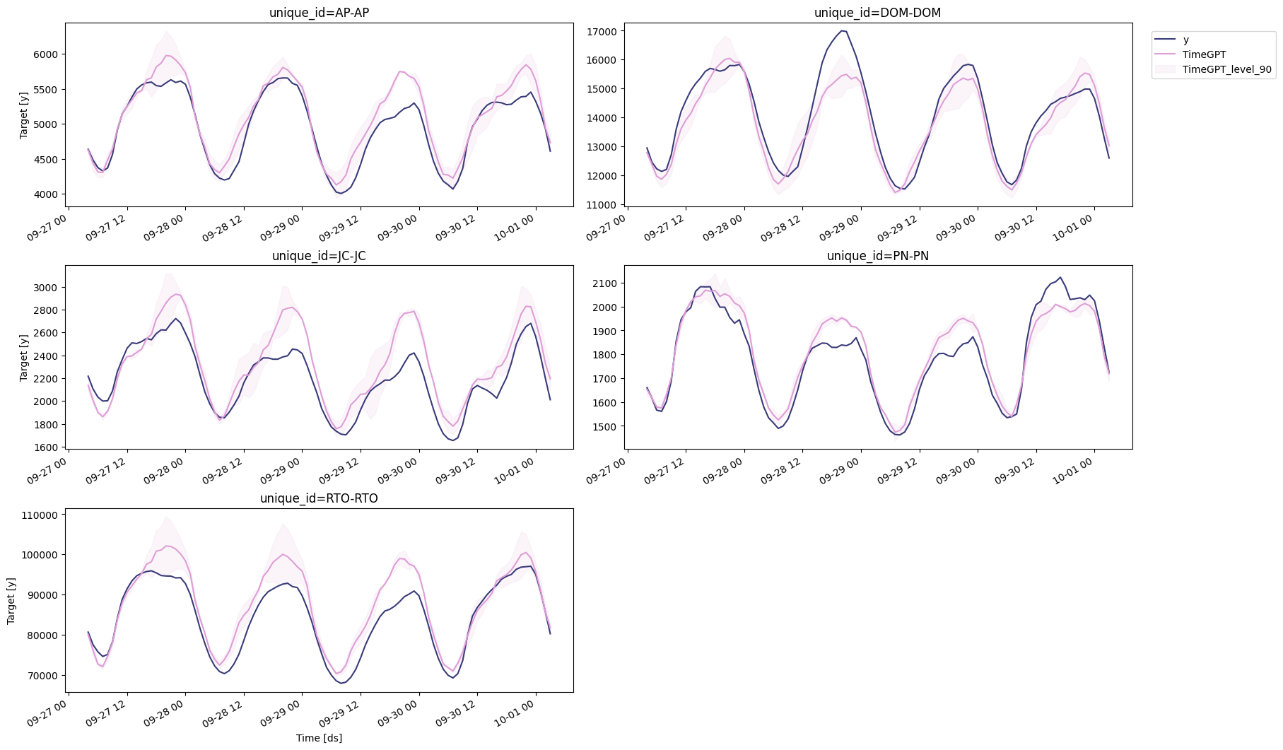
The first step is to split our data. Here, we define an input DataFrame to feed to the model. We also reserve the last 96 time steps for the test set, so that we can evaluate the performance of TimeGPT against actual values. For this situation, we use a forecast horizon of 96, which represents four days, and we use an input sequence of 362 days, which is 8688 time steps.Forecasting
Then, we simply call theforecast method. Here, we use fine-tuning and
specify the mean absolute error (MAE) as the fine-tuning loss. Also, we
use the timegpt-1-long-horizon since we are forecasting the next two
days, and the seasoanl period is one day.
📘 Available models in Azure AI If you are using an Azure AI endpoint, please be sure to setTimeGPT was done in 4.3 seconds! We can now plot the predictions against the actual values of the test set.model="azureai":nixtla_client.forecast(..., model="azureai")For the public API, we support two models:timegpt-1andtimegpt-1-long-horizon. By default,timegpt-1is used. Please see this tutorial on how and when to usetimegpt-1-long-horizon.
Evaluation
Now that we have predictions, let’s evaluate the model’s performance.Forecasting with N-HiTS
Here, we use the N-HiTS model, as it is very fast to train and performs well on long-horizon forecasting tasks. To reproduce these results, make sure to install the libraryneuralforecast.