

Initial setup
We start off by importing the required packages for this tutorial and create an instace ofNixtlaClient.
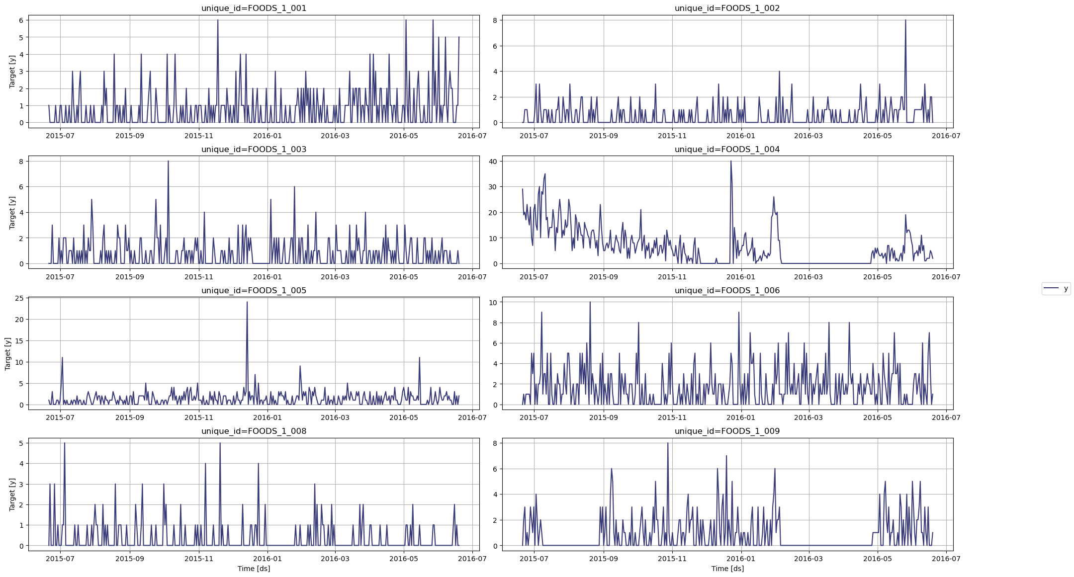
👍 Use an Azure AI endpoint To use an Azure AI endpoint, remember to set also theWe now read the dataset and plot it.base_urlargument:nixtla_client = NixtlaClient(base_url="you azure ai endpoint", api_key="your api_key")
| unique_id | ds | y | sell_price | event_type_Cultural | event_type_National | event_type_Religious | event_type_Sporting | |
|---|---|---|---|---|---|---|---|---|
| 0 | FOODS_1_001 | 2011-01-29 | 3 | 2.0 | 0 | 0 | 0 | 0 |
| 1 | FOODS_1_001 | 2011-01-30 | 0 | 2.0 | 0 | 0 | 0 | 0 |
| 2 | FOODS_1_001 | 2011-01-31 | 0 | 2.0 | 0 | 0 | 0 | 0 |
| 3 | FOODS_1_001 | 2011-02-01 | 1 | 2.0 | 0 | 0 | 0 | 0 |
| 4 | FOODS_1_001 | 2011-02-02 | 4 | 2.0 | 0 | 0 | 0 | 0 |
Bounded forecasts
To avoid getting negative predictions coming from the model, we use a log transformation on the data. That way, the model will be forced to predict only positive values. Note that due to the presence of zeros in our dataset, we add one to all points before taking the log.| unique_id | ds | y | sell_price | event_type_Cultural | event_type_National | event_type_Religious | event_type_Sporting | |
|---|---|---|---|---|---|---|---|---|
| 0 | FOODS_1_001 | 2011-01-29 | 1.386294 | 2.0 | 0 | 0 | 0 | 0 |
| 1 | FOODS_1_001 | 2011-01-30 | 0.000000 | 2.0 | 0 | 0 | 0 | 0 |
| 2 | FOODS_1_001 | 2011-01-31 | 0.000000 | 2.0 | 0 | 0 | 0 | 0 |
| 3 | FOODS_1_001 | 2011-02-01 | 0.693147 | 2.0 | 0 | 0 | 0 | 0 |
| 4 | FOODS_1_001 | 2011-02-02 | 1.609438 | 2.0 | 0 | 0 | 0 | 0 |
Forecasting with TimeGPT
📘 Available models in Azure AI If you are using an Azure AI endpoint, please be sure to setGreat! TimeGPT was done in 5.8 seconds and we now have predictions. However, those predictions are transformed, so we need to inverse the transformation to get back to the orignal scale. Therefore, we take the exponential and subtract one from each data point.model="azureai":nixtla_client.forecast(..., model="azureai")For the public API, we support two models:timegpt-1andtimegpt-1-long-horizon. By default,timegpt-1is used. Please see this tutorial on how and when to usetimegpt-1-long-horizon.
| unique_id | ds | TimeGPT | TimeGPT-lo-80 | TimeGPT-hi-80 | |
|---|---|---|---|---|---|
| 0 | FOODS_1_001 | 2016-05-23 | 0.286841 | -0.267101 | 1.259465 |
| 1 | FOODS_1_001 | 2016-05-24 | 0.320482 | -0.241236 | 1.298046 |
| 2 | FOODS_1_001 | 2016-05-25 | 0.287392 | -0.362250 | 1.598791 |
| 3 | FOODS_1_001 | 2016-05-26 | 0.295326 | -0.145489 | 0.963542 |
| 4 | FOODS_1_001 | 2016-05-27 | 0.315868 | -0.166516 | 1.077437 |
Evaluation
Before measuring the performance metric, let’s plot the predictions against the actual values.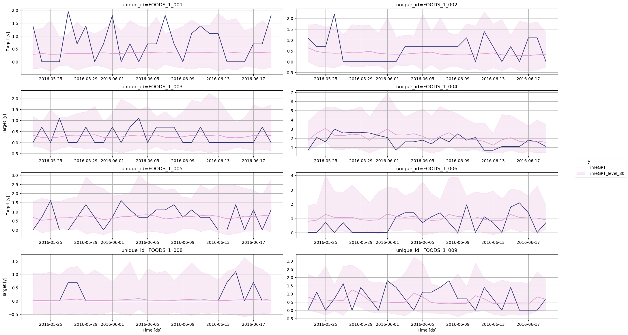
Forecasting with statistical models
The librarystatsforecast by Nixtla provides a suite of statistical
models specifically built for intermittent forecasting, such as Croston,
IMAPA and TSB. Let’s use these models and see how they perform against
TimeGPT.
| ds | CrostonClassic | CrostonOptimized | IMAPA | TSB | |
|---|---|---|---|---|---|
| unique_id | |||||
| FOODS_1_001 | 2016-05-23 | 0.599093 | 0.599093 | 0.445779 | 0.396258 |
| FOODS_1_001 | 2016-05-24 | 0.599093 | 0.599093 | 0.445779 | 0.396258 |
| FOODS_1_001 | 2016-05-25 | 0.599093 | 0.599093 | 0.445779 | 0.396258 |
| FOODS_1_001 | 2016-05-26 | 0.599093 | 0.599093 | 0.445779 | 0.396258 |
| FOODS_1_001 | 2016-05-27 | 0.599093 | 0.599093 | 0.445779 | 0.396258 |
Evaluation
Now, let’s combine the predictions from all methods and see which performs best.| unique_id | ds | y | sell_price | event_type_Cultural | event_type_National | event_type_Religious | event_type_Sporting | TimeGPT | TimeGPT-lo-80 | TimeGPT-hi-80 | CrostonClassic | CrostonOptimized | IMAPA | TSB | |
|---|---|---|---|---|---|---|---|---|---|---|---|---|---|---|---|
| 0 | FOODS_1_001 | 2016-05-23 | 1.386294 | 2.24 | 0 | 0 | 0 | 0 | 0.286841 | -0.267101 | 1.259465 | 0.599093 | 0.599093 | 0.445779 | 0.396258 |
| 1 | FOODS_1_001 | 2016-05-24 | 0.000000 | 2.24 | 0 | 0 | 0 | 0 | 0.320482 | -0.241236 | 1.298046 | 0.599093 | 0.599093 | 0.445779 | 0.396258 |
| 2 | FOODS_1_001 | 2016-05-25 | 0.000000 | 2.24 | 0 | 0 | 0 | 0 | 0.287392 | -0.362250 | 1.598791 | 0.599093 | 0.599093 | 0.445779 | 0.396258 |
| 3 | FOODS_1_001 | 2016-05-26 | 0.000000 | 2.24 | 0 | 0 | 0 | 0 | 0.295326 | -0.145489 | 0.963542 | 0.599093 | 0.599093 | 0.445779 | 0.396258 |
| 4 | FOODS_1_001 | 2016-05-27 | 1.945910 | 2.24 | 0 | 0 | 0 | 0 | 0.315868 | -0.166516 | 1.077437 | 0.599093 | 0.599093 | 0.445779 | 0.396258 |
| TimeGPT | CrostonClassic | CrostonOptimized | IMAPA | TSB | |
|---|---|---|---|---|---|
| metric | |||||
| mae | 0.492559 | 0.564563 | 0.580922 | 0.571943 | 0.567178 |
Forecasting with exogenous variables using TimeGPT
To forecast with exogenous variables, we need to specify their future values over the forecast horizon. Therefore, let’s simply take the types of events, as those dates are known in advance.| unique_id | ds | event_type_Cultural | event_type_National | event_type_Religious | event_type_Sporting | |
|---|---|---|---|---|---|---|
| 0 | FOODS_1_001 | 2016-05-23 | 0 | 0 | 0 | 0 |
| 1 | FOODS_1_001 | 2016-05-24 | 0 | 0 | 0 | 0 |
| 2 | FOODS_1_001 | 2016-05-25 | 0 | 0 | 0 | 0 |
| 3 | FOODS_1_001 | 2016-05-26 | 0 | 0 | 0 | 0 |
| 4 | FOODS_1_001 | 2016-05-27 | 0 | 0 | 0 | 0 |
forecast method and pass the futr_exog_df
in the X_df parameter.
📘 Available models in Azure AI If you are using an Azure AI endpoint, please be sure to setGreat! Remember that the predictions are transformed, so we have to inverse the transformation again.model="azureai":nixtla_client.forecast(..., model="azureai")For the public API, we support two models:timegpt-1andtimegpt-1-long-horizon. By default,timegpt-1is used. Please see this tutorial on how and when to usetimegpt-1-long-horizon.
| unique_id | ds | TimeGPT_ex | TimeGPT-lo-80 | TimeGPT-hi-80 | |
|---|---|---|---|---|---|
| 0 | FOODS_1_001 | 2016-05-23 | 0.281922 | -0.269902 | 1.250828 |
| 1 | FOODS_1_001 | 2016-05-24 | 0.313774 | -0.245091 | 1.286372 |
| 2 | FOODS_1_001 | 2016-05-25 | 0.285639 | -0.363119 | 1.595252 |
| 3 | FOODS_1_001 | 2016-05-26 | 0.295037 | -0.145679 | 0.963104 |
| 4 | FOODS_1_001 | 2016-05-27 | 0.315484 | -0.166760 | 1.076830 |
Evaluation
Finally, let’s evaluate the performance of TimeGPT with exogenous features.| unique_id | ds | y | sell_price | event_type_Cultural | event_type_National | event_type_Religious | event_type_Sporting | TimeGPT | TimeGPT-lo-80 | TimeGPT-hi-80 | CrostonClassic | CrostonOptimized | IMAPA | TSB | TimeGPT_ex | |
|---|---|---|---|---|---|---|---|---|---|---|---|---|---|---|---|---|
| 0 | FOODS_1_001 | 2016-05-23 | 1.386294 | 2.24 | 0 | 0 | 0 | 0 | 0.286841 | -0.267101 | 1.259465 | 0.599093 | 0.599093 | 0.445779 | 0.396258 | 0.281922 |
| 1 | FOODS_1_001 | 2016-05-24 | 0.000000 | 2.24 | 0 | 0 | 0 | 0 | 0.320482 | -0.241236 | 1.298046 | 0.599093 | 0.599093 | 0.445779 | 0.396258 | 0.313774 |
| 2 | FOODS_1_001 | 2016-05-25 | 0.000000 | 2.24 | 0 | 0 | 0 | 0 | 0.287392 | -0.362250 | 1.598791 | 0.599093 | 0.599093 | 0.445779 | 0.396258 | 0.285639 |
| 3 | FOODS_1_001 | 2016-05-26 | 0.000000 | 2.24 | 0 | 0 | 0 | 0 | 0.295326 | -0.145489 | 0.963542 | 0.599093 | 0.599093 | 0.445779 | 0.396258 | 0.295037 |
| 4 | FOODS_1_001 | 2016-05-27 | 1.945910 | 2.24 | 0 | 0 | 0 | 0 | 0.315868 | -0.166516 | 1.077437 | 0.599093 | 0.599093 | 0.445779 | 0.396258 | 0.315484 |
| TimeGPT | CrostonClassic | CrostonOptimized | IMAPA | TSB | TimeGPT_ex | |
|---|---|---|---|---|---|---|
| metric | ||||||
| mae | 0.492559 | 0.564563 | 0.580922 | 0.571943 | 0.567178 | 0.485352 |