

Quantify uncertaintyProbabilistic forecasting is a natural answer to quantify the uncertainty of target variable’s future. The task requires to model the following conditional predictive distribution: We will show you how to tackle the task with
NeuralForecast by
combining a classic Long Short Term Memory Network
(LSTM) and the Neural Hierarchical
Interpolation (NHITS) with the multi
quantile loss function (MQLoss).
In this notebook we will:1. Install NeuralForecast Library
2. Explore the M4-Hourly data.
3. Train the LSTM and NHITS
4. Visualize the LSTM/NHITS prediction intervals. You can run these experiments using GPU with Google Colab.
1. Installing NeuralForecast
Useful functions
Theplot_grid auxiliary function defined below will be useful to plot
different time series, and different models’ forecasts.
2. Loading M4 Data
For testing purposes, we will use the Hourly dataset from the M4 competition.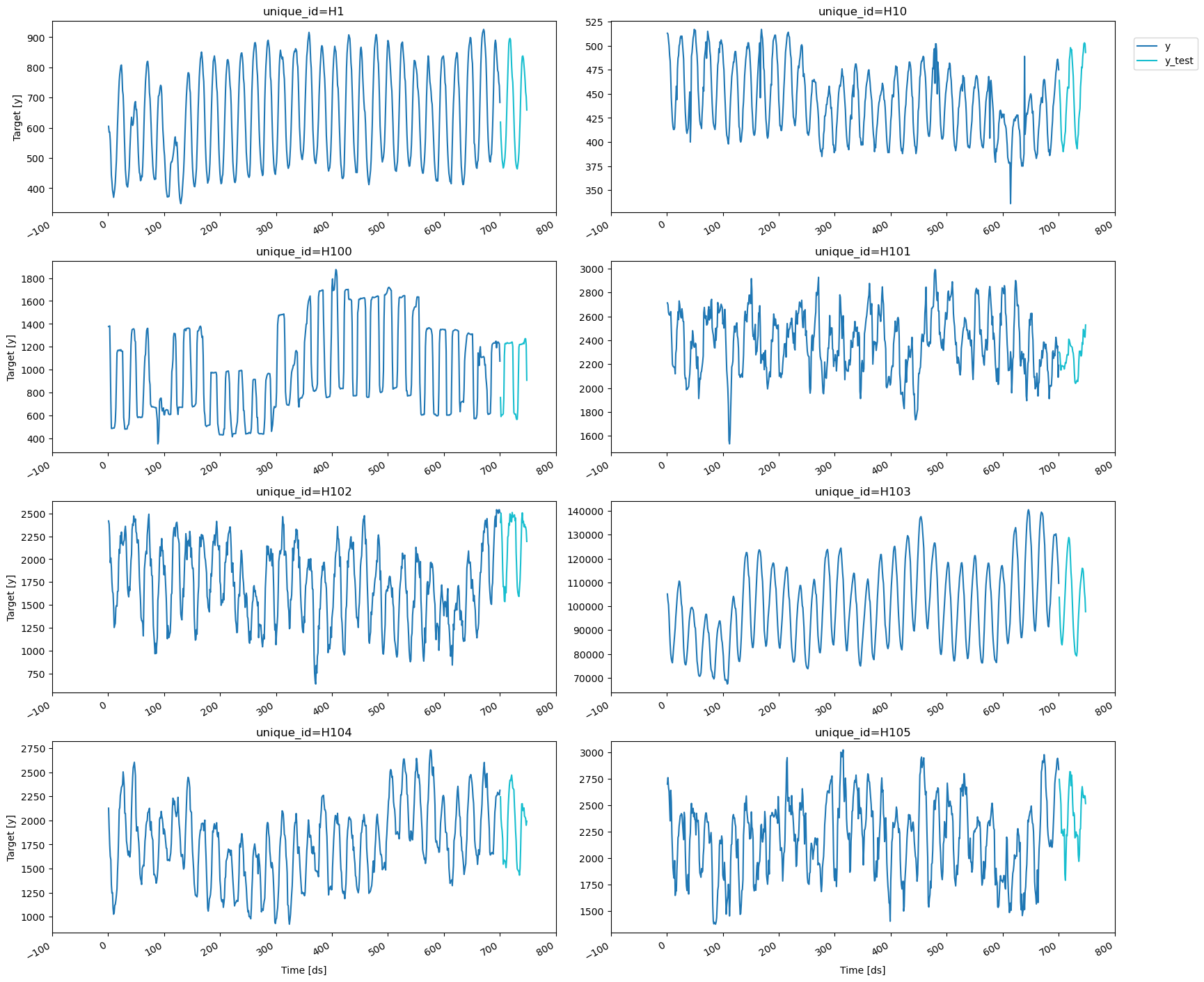
3. Model Training
Thecore.NeuralForecast provides a high-level interface with our
collection of PyTorch models. NeuralForecast is instantiated with a
list of models=[LSTM(...), NHITS(...)], configured for the forecasting
task.
- The
horizonparameter controls the number of steps ahead of the predictions, in this example 48 hours ahead (2 days). - The
MQLosswithlevels=[80,90]specializes the network’s output into the 80% and 90% prediction intervals. - The
max_steps=2000, controls the duration of the network’s training.
Y_train_df is used during a shared optimization to train a single
model with shared parameters. This is the most common practice in the
forecasting literature for deep learning models, and it is known as
“cross-learning”.
| unique_id | ds | LSTM-median | LSTM-lo-90 | LSTM-lo-80 | LSTM-hi-80 | LSTM-hi-90 | NHITS-median | NHITS-lo-90 | NHITS-lo-80 | NHITS-hi-80 | NHITS-hi-90 | |
|---|---|---|---|---|---|---|---|---|---|---|---|---|
| 0 | H1 | 701 | 650.919861 | 526.705933 | 551.696289 | 748.392456 | 777.889526 | 615.786743 | 582.732117 | 584.717468 | 640.011841 | 647.147034 |
| 1 | H1 | 702 | 547.724487 | 439.353394 | 463.725464 | 638.429626 | 663.398987 | 569.632324 | 524.486023 | 522.324402 | 578.411560 | 594.515076 |
| 2 | H1 | 703 | 514.851074 | 421.289917 | 443.166443 | 589.451782 | 608.560425 | 518.858887 | 503.183411 | 501.016968 | 536.081543 | 549.701050 |
| 3 | H1 | 704 | 485.141418 | 403.336914 | 421.090546 | 547.966492 | 567.057800 | 495.627869 | 476.579742 | 468.514069 | 498.171600 | 527.931091 |
| 4 | H1 | 705 | 462.695831 | 383.011108 | 399.126282 | 522.579224 | 543.981750 | 481.584534 | 468.134857 | 472.723450 | 496.198975 | 513.859985 |
4. Plotting Predictions
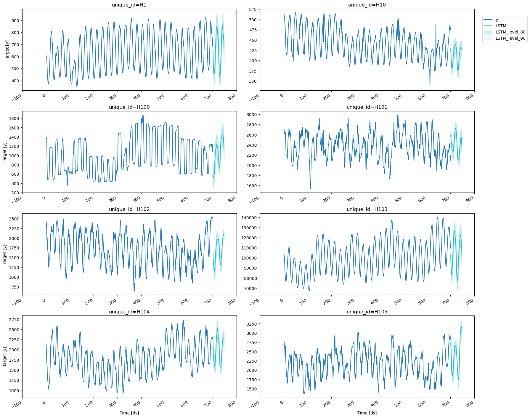
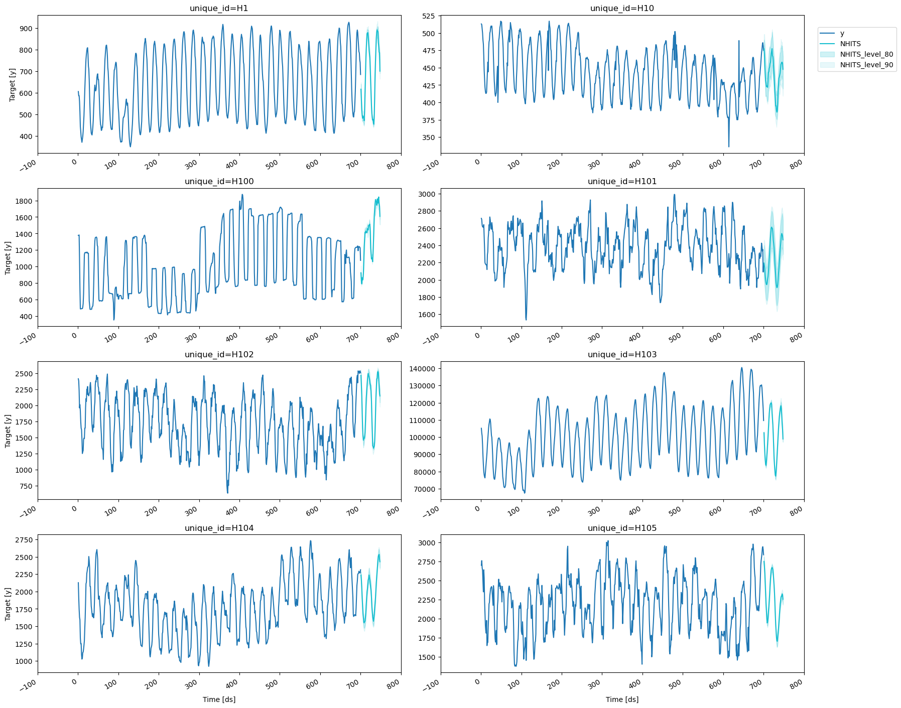
Here we finalize our analysis by plotting the prediction intervals and verifying that both theLSTM and NHITS are giving excellent results.
Consider the output [NHITS-lo-90.0, NHITS-hi-90.0], that represents
the 80% prediction interval of the NHITS network; its lower limit
gives the 5th percentile (or 0.05 quantile) while its upper limit gives
the 95th percentile (or 0.95 quantile). For well-trained models we
expect that the target values lie within the interval 90% of the time.
LSTM
NHITS
References
- Roger Koenker and Gilbert Basset (1978). Regression Quantiles,
Econometrica.
- Jeffrey L. Elman (1990). “Finding Structure in
Time”.
- Cristian Challu, Kin G. Olivares, Boris N. Oreshkin, Federico
Garza, Max Mergenthaler-Canseco, Artur Dubrawski (2021). NHITS:
Neural Hierarchical Interpolation for Time Series Forecasting.
Accepted at AAAI 2023.