Sequential predictive conformal inference

The residual-based methods take their width from a quantile of past errors, so at a given horizon step it is a constant. SPCI fits a quantile regressor on the recent residual history and predicts the next residual’s spread instead, so the width moves with the state the series is in.

What it does

For each (series, horizon) cell, SPCI fits a quantile regressor that predicts the next signed residual from the previous window_size residuals — and from exogenous features, if you supply them. Call its predicted quantile function Q. The interval is

[ŷ + Q(beta), ŷ + Q(1 - alpha + beta)]

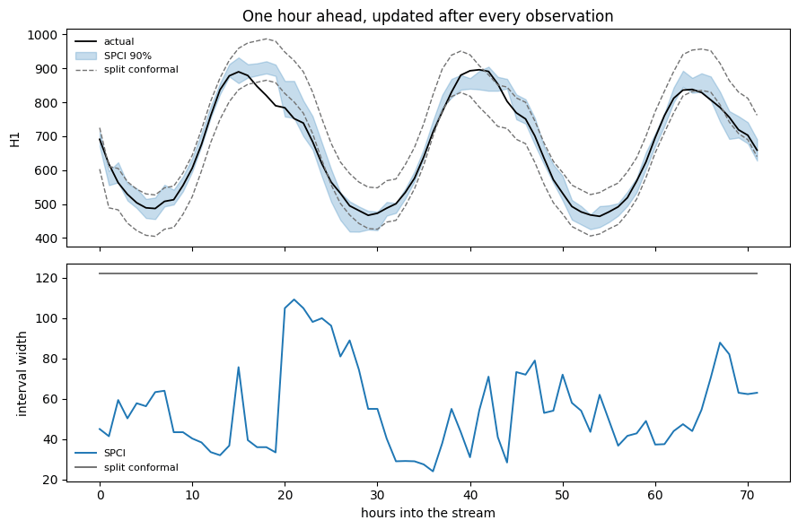
for whichever beta in [0, alpha] makes it narrowest. That search is the second idea: an interval of the right coverage need not be centred. When the residual distribution is skewed, spending more of alpha on one tail gives a tighter interval at the same nominal level, and SPCI searches a grid of beta_grid_size candidates for the best split. Because Q depends on the recent residual history, the width moves with the data. A run of large errors widens the next interval directly, without waiting for a controller to notice a miss.

Original method The paper’s estimator is a quantile random forest, which is also this implementation’s default.

SPCI needs the spci extra and costs more than the others The default QRFQuantileRegressor wraps quantile-forest: pip install conformalforecast[spci]. SPCI is also the one sanctioned exception to the package’s no-per-cell-loops rule — it fits one regressor per (series, horizon) cell, so an 8-series panel at horizon 24 means 192 forests. Keep the grid small, or raise refit_every so the regressors are refitted less often.

Worked example

SPCI is formulated for sequential one-step-ahead prediction, so that is what this page does: forecast one hour ahead on a single M4 hourly series, and stream three days through the method an observation at a time.

import matplotlib.pyplot as plt
import numpy as np
import pandas as pd
from statsforecast import StatsForecast
from statsforecast.models import SeasonalNaive

from conformalforecast import SequentialPredictiveConformalInference, SplitConformal
from conformalforecast.adapters import StatsForecastAdapter
from conformalforecast.diagnostics import spci_state

SEASON, ALPHA, WINDOW = 24, 0.1, 48
N_STREAM = 72  # three days, one hour at a time

full = pd.read_csv("nbs/data/m4_hourly_panel.csv", parse_dates=["ds"])
df = full[full["unique_id"] == "H1"].reset_index(drop=True)
series = df["y"].to_numpy()[None, :]
train_end = series.shape[1] - N_STREAM
train_df = df.iloc[:train_end].reset_index(drop=True)

sf = StatsForecast(models=[SeasonalNaive(season_length=SEASON)], freq="h", n_jobs=1)
sf.fit(train_df)
forecaster = StatsForecastAdapter(
    sf=sf, train_df=train_df, horizon=1, freq="h", model_name="SeasonalNaive"
)

spci = SequentialPredictiveConformalInference(alpha=ALPHA, window_size=WINDOW, refit_every=4)
spci_fitted = spci.calibrate_cv(forecaster, n_windows=150, refit=True)

split_fitted = SplitConformal(alpha=ALPHA).calibrate_cv(forecaster, n_windows=150, refit=True)

state = spci_state(spci_fitted)
for key in ("window_size", "n_observations", "n_regressors", "regressor_class", "refit_every"):
    print(f"{key:18s} {state[key]}")

window_size        48
n_observations     150
n_regressors       1
regressor_class    QRFQuantileRegressor
refit_every        4

n_regressors is the (series × horizon) grid — one series, one horizon step, so one forest. Each saw n_observations residuals and keeps the last window_size of them as its feature vector.

SPCI needs a longer calibration set than the others The minimum is max(window_size + 1, ceil(1/alpha)) effective residuals per series, not just ceil(1/alpha) — the regressor needs a full window before it can predict anything. That is why this page asks for 150 cross-validation windows where the split conformal page needed 24.

def stream(fitted, *, online=True):
    """Roll one hour at a time, recording the interval and whether it covered."""
    lower, upper, covered = [], [], []
    for t in range(train_end, series.shape[1]):
        prediction = fitted.predict(series[:, :t])
        lo, hi = prediction.interval[0, 0, 0]
        lower.append(lo)
        upper.append(hi)
        covered.append(lo <= series[0, t] <= hi)
        if online:
            fitted.update(prediction.point, series[:, t : t + 1][:, None, :])
    return {"lower": np.array(lower), "upper": np.array(upper), "covered": np.array(covered)}


runs = {"SPCI": stream(spci_fitted), "split conformal": stream(split_fitted, online=False)}

for name, run in runs.items():
    width = run["upper"] - run["lower"]
    print(
        f"{name:18s} coverage {run['covered'].mean():6.1%}   "
        f"mean width {width.mean():7.1f}   "
        f"width range {width.min():6.1f} - {width.max():6.1f}"
    )

SPCI               coverage  81.9%   mean width    55.1   width range   24.0 -  109.3
split conformal    coverage  79.2%   mean width   122.0   width range  122.0 -  122.0

Width that moves

hours = np.arange(N_STREAM)
truth = series[0, train_end:]

fig, (top, bottom) = plt.subplots(2, 1, figsize=(9, 6), sharex=True)

top.plot(hours, truth, color="k", lw=1.3, label="actual")
top.fill_between(
    hours,
    runs["SPCI"]["lower"],
    runs["SPCI"]["upper"],
    color="C0",
    alpha=0.25,
    label="SPCI 90%",
)
top.plot(
    hours, runs["split conformal"]["lower"], color="0.45", lw=1, ls="--", label="split conformal"
)
top.plot(hours, runs["split conformal"]["upper"], color="0.45", lw=1, ls="--")
top.set_ylabel("H1")
top.set_title("One hour ahead, updated after every observation")
top.legend(fontsize=8, frameon=False, loc="upper left")

for name, colour in [("SPCI", "C0"), ("split conformal", "0.45")]:
    bottom.plot(hours, runs[name]["upper"] - runs[name]["lower"], color=colour, lw=1.4, label=name)
bottom.set_ylabel("interval width")
bottom.set_xlabel("hours into the stream")
bottom.legend(fontsize=8, frameon=False)
fig.tight_layout()

The bottom panel is the whole argument. Split conformal draws a horizontal line — its width is a constant of the fitted state, identical at 3 a.m. and at the evening peak. SPCI’s width rises and falls, because the residuals it regresses on do. Both are valid intervals. Only one of them is informative: a width that carries a signal tells you something the point forecast does not. Here that pays on both axes at once. SPCI covered 82% of the stream at a mean width of 55, while split conformal covered 79% at a constant width of 122 — less than half the width for slightly better coverage. Note that neither reached the 90% target over these particular 72 hours; three days is a short measurement, and the widest SPCI intervals cluster exactly where the series ramps.

Measure SPCI’s coverage before you trust it SPCI’s validity is asymptotic and conditional on the residual model being reasonable, which is a much weaker footing than split conformal’s finite-sample guarantee. Two consequences show up in practice:

Even on well-behaved data it tends to land a few points below nominal. The package’s own coverage test (tests/unit/methods/test_spci.py) allows a tolerance of 0.08 around the target for exactly this reason.

At multi-step horizons on real series the gap can be much larger. On this same panel at horizon 6, SPCI covers around 65% against a 90% target while split conformal holds 90% — the quantile forest is asked to extrapolate to residual magnitudes it never saw in training, and tree models cannot extrapolate.

Neither is a reason to avoid SPCI; both are reasons to run evaluate on your own data and horizon before shipping it, rather than assuming the guarantee carries over.

When not to use it

You cannot install the extra. SPCI is the only method with a third-party dependency.
Your grid is large. n_series × horizon regressors, refitted as you go. A 100-series panel at horizon 48 is 4 800 forests — consider CQR, which gets varying width from a model you already fit.
Your calibration set is short. window_size + 1 residuals per series is a real constraint, and the default window_size is 100.
You need the classical guarantee, or a long horizon. Split conformal is finite-sample and assumption-light; on this data it is also the one that holds its coverage at horizon 6.

References

C. Xu and Y. Xie, “Sequential Predictive Conformal Inference for Time Series,” in Proc. ICML, 2023. https://arxiv.org/abs/2212.03463.

Methods overview — the decision guide, now that you have seen all seven.
Exogenous features — SPCI is the method that can actually use them.
Diagnostics — how to run the measurement the callout above asks for.

Getting Started

Concepts

Capabilities

Methods

Nixtlaverse

API Reference

Sequential predictive conformal inference

What it does

Worked example

Width that moves

When not to use it

References

Next

​What it does

​Worked example

​Width that moves

​When not to use it

​References

​Next

What it does

Worked example

Width that moves

When not to use it

References

Next