Nonexchangeable conformal prediction

NexCP answers the same problem as ACI — the world moved and the calibration set is stale — from the opposite direction. Rather than moving the coverage target, it changes whose errors count.

What it does

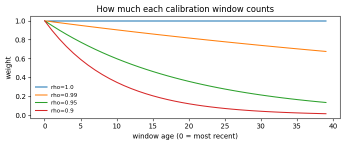
Split conformal treats all n calibration windows as equally informative, which is precisely the exchangeability assumption. NexCP drops it and weights each window by its age:

w_i = rho ** (age of window i)

The newest window has weight 1, the one before it rho, and so on. The threshold is then the exact weighted order statistic of the scores under those weights, not the unweighted one. rho controls the memory. At rho = 1 every weight is 1 and NexCP is exactly split conformal. At rho = 0.9 a window 20 steps back carries 12% of the newest window’s vote, and one 50 steps back is essentially ignored. Barber et al. give the price explicitly: the coverage gap is bounded by the total variation between the weighted calibration distribution and the test point’s. Down-weighting stale data shrinks that gap when the process drifts, and costs you effective sample size when it does not.

The window axis has to mean time NexCP reads axis 1 of the calibration arrays as chronological, oldest first. That is what calibrate_cv produces. If you assemble calibration windows yourself, get the order right or the decay is applied to the wrong windows silently.

Worked example

This page uses the eight-series M4 hourly panel rather than AirPassengers, because weighting only matters when the series are long enough for old windows to genuinely be stale.

import matplotlib.pyplot as plt
import numpy as np
import pandas as pd
from statsforecast import StatsForecast
from statsforecast.models import SeasonalNaive

from conformalforecast import NonexchangeableConformalPrediction
from conformalforecast import panel as P
from conformalforecast.adapters import StatsForecastAdapter
from conformalforecast.diagnostics import evaluate, nexcp_state

HORIZON, SEASON, ALPHA = 24, 24, 0.1
N_HOLDOUT = 3

df = pd.read_csv("nbs/data/m4_hourly_panel.csv", parse_dates=["ds"])
matrix, index = P.long_to_panel(df["y"].to_numpy(), df["unique_id"].to_numpy(), df["ds"].to_numpy())
print("panel", matrix.shape, "series", index.series_ids)

# Hold the tail out before anything is fitted, so the coverage measured at the
# end of this page is measured on data no part of the pipeline has seen.
train_df = df[df["ds"] <= df["ds"].max() - pd.Timedelta(hours=N_HOLDOUT * HORIZON)].reset_index(
    drop=True
)
print("training through", train_df["ds"].max(), f"({N_HOLDOUT * HORIZON} hours held out)")

sf = StatsForecast(models=[SeasonalNaive(season_length=SEASON)], freq="h", n_jobs=1)
sf.fit(train_df)
forecaster = StatsForecastAdapter(
    sf=sf, train_df=train_df, horizon=HORIZON, freq="h", model_name="SeasonalNaive"
)

panel (8, 672) series ('H1', 'H10', 'H100', 'H150', 'H200', 'H300', 'H400', 'H50')
training through 2015-01-25 23:00:00 (72 hours held out)

refit=True for SeasonalNaive SeasonalNaive has no forward method, so statsforecast cannot reuse fitted parameters across cutoffs and calibrate_cv must refit at each one. For this model that is free — there is nothing to fit.

N_WINDOWS = 40
RHOS = [1.0, 0.99, 0.95, 0.9]

fits, states = {}, {}
for rho in RHOS:
    method = NonexchangeableConformalPrediction(alpha=ALPHA, rho=rho)
    fits[rho] = method.calibrate_cv(forecaster, n_windows=N_WINDOWS, refit=True)
    states[rho] = nexcp_state(fits[rho])

for rho, state in states.items():
    label = "rho=1.0 (= split conformal)" if rho == 1.0 else f"rho={rho}"
    print(
        f"{label:28s} effective sample size {state['effective_sample_size']:6.2f}"
        f"   of {N_WINDOWS} windows"
    )

rho=1.0 (= split conformal)  effective sample size  40.00   of 40 windows
rho=0.99                     effective sample size  39.47   of 40 windows
rho=0.95                     effective sample size  30.12   of 40 windows
rho=0.9                      effective sample size  18.45   of 40 windows

The effective sample size is what the decay costs. rho = 0.99 is almost free here — 39.5 of 40 windows — while rho = 0.9 leaves the equivalent of about 18. Fewer effective windows means a coarser quantile grid and a noisier threshold. That is the trade: less stale information, but also less information.

ages = np.arange(N_WINDOWS)
fig, ax = plt.subplots(figsize=(7, 3))
for i, rho in enumerate(RHOS):
    ax.plot(ages, np.power(rho, ages), color=f"C{i}", lw=1.5, label=f"rho={rho}")
ax.set_xlabel("window age (0 = most recent)")
ax.set_ylabel("weight")
ax.set_title("How much each calibration window counts")
ax.legend(fontsize=8, frameon=False)
fig.tight_layout()

What it does to the intervals

predictions = {rho: fits[rho].predict(matrix) for rho in RHOS}

series = 0
steps = np.arange(1, HORIZON + 1)
fig, ax = plt.subplots(figsize=(9, 3.8))
for i, rho in enumerate(RHOS):
    interval = predictions[rho].interval[series, 0]
    label = "rho=1.0 (split conformal)" if rho == 1.0 else f"rho={rho}"
    ax.plot(steps, interval[:, 0], color=f"C{i}", lw=1.3, label=label)
    ax.plot(steps, interval[:, 1], color=f"C{i}", lw=1.3)
ax.plot(steps, predictions[1.0].point[series, 0], color="k", lw=1.4, ls="--", label="forecast")
ax.set_xlabel("horizon (hours ahead)")
ax.set_ylabel(f"{index.series_ids[series]}")
ax.set_title("Faster decay, different band")
ax.legend(fontsize=8, frameon=False, ncol=2)
fig.tight_layout()

widths = {
    rho: (predictions[rho].interval[..., 1] - predictions[rho].interval[..., 0]).mean(axis=(1, 2))
    for rho in RHOS
}
header = "series   " + "".join(f"{('rho=' + str(r)):>12s}" for r in RHOS)
print(header)
for s, name in enumerate(index.series_ids):
    row = "".join(f"{widths[rho][s]:12.1f}" for rho in RHOS)
    print(f"{name:9s}{row}")

series        rho=1.0    rho=0.99    rho=0.95     rho=0.9
H1              140.0       146.7       155.0       165.3
H10              44.4        63.3       110.9       199.8
H100            539.5       610.9       666.8       811.3
H150            179.9       206.5       217.4       257.4
H200              0.4         0.4         0.4         0.4
H300              0.5         0.5         0.6         0.6
H400             89.3        93.8       133.2       205.0
H50            8804.0      8829.0      8829.8      9336.3

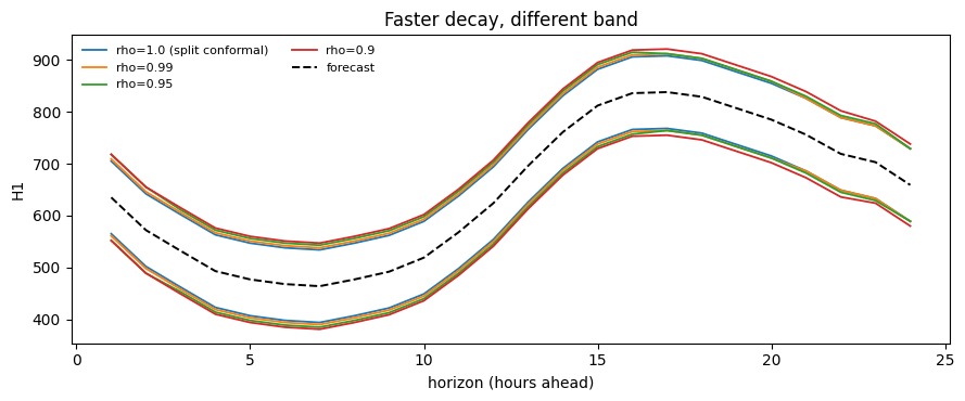
The widths move by series, not uniformly: rho reweights each series’ own residual history, so a series whose recent errors are unlike its old ones changes a lot — H10 more than quadruples between rho = 1.0 and rho = 0.9 — while a stable one such as H200 barely moves. A single global multiplier could not do that.

Measured coverage

histories, truths = [], []
for k in range(N_HOLDOUT):
    end = matrix.shape[1] - (N_HOLDOUT - k) * HORIZON
    histories.append(matrix[:, :end])
    truths.append(matrix[:, end : end + HORIZON])
truths = np.stack(truths, axis=1)

for rho in RHOS:
    report = evaluate(fits[rho], histories, truths)
    label = "rho=1.0 (split)" if rho == 1.0 else f"rho={rho}"
    print(
        f"{label:18s} coverage {report.marginal_coverage:6.1%}   "
        f"width {report.mean_interval_width:9.1f}   "
        f"Winkler {report.mean_winkler_score:9.1f}"
    )

rho=1.0 (split)    coverage  85.9%   width    1227.7   Winkler    1369.0
rho=0.99           coverage  89.4%   width    1241.2   Winkler    1360.8
rho=0.95           coverage  92.5%   width    1263.8   Winkler    1338.8
rho=0.9            coverage  94.8%   width    1371.3   Winkler    1429.2

The decay pays for itself here, up to a point Split conformal (rho = 1.0) under-covers on this holdout — 85.9% against a 90% target — because it weights a residual from 40 hours back exactly as heavily as the most recent one. Every decay setting closes that gap, rho = 0.99 almost exactly (89.4%), and the Winkler score, which charges width and misses on one scale, improves with it, bottoming out at rho = 0.95 (1338.8 against split’s 1369.0). Past that the trade turns over. rho = 0.9 buys 94.8% coverage, well beyond what was asked for, and pays 12% more width than split conformal to get it; its Winkler score is the worst of the four. That is the shape to expect — forgetting stale residuals helps while they really are misleading, and costs you effective sample size once they are not. Measure before tuning rho, in both directions.

When not to use it

Your calibration set is small. Decay throws away effective sample size you may not have. Check effective_sample_size against ceil(1/alpha) before trusting the result.
Your drift is abrupt rather than gradual. An exponential decay is a smooth forgetting curve. A step change is handled better by ACI, whose controller reacts to misses directly.
You do not know how fast to forget. rho is as much a tuning parameter as ACI’s gamma, and NexCP has no aggregated variant. If that bothers you, use AgACI.

References

R. F. Barber, E. J. Candes, A. Ramdas, and R. J. Tibshirani, “Conformal prediction beyond exchangeability,” arXiv.org, 2022. https://arxiv.org/abs/2202.13415.

SPCI — the last online method, and the only one that changes the shape of the band rather than its level.
Ragged panels — what the window axis means when series have different lengths, which is exactly what NexCP reads.

Getting Started

Concepts

Capabilities

Methods

Nixtlaverse

API Reference

Nonexchangeable conformal prediction

What it does

Worked example

What it does to the intervals

Measured coverage

When not to use it

References

Next

​What it does

​Worked example

​What it does to the intervals

​Measured coverage

​When not to use it

​References

​Next

What it does

Worked example

What it does to the intervals

Measured coverage

When not to use it

References

Next