Quick start

conformalforecast turns a point forecaster into one that emits calibrated prediction intervals. This page goes from a CSV to a 90% interval with a measured coverage rate, using statsforecast and split conformal prediction. Nothing here is specific to statsforecast. The same five steps work for mlforecast, neuralforecast, or a function you wrote yourself — only the adapter in step 2 changes.

1. The data

AirPassengers: monthly international airline passengers, from 1949 to 1960.

import matplotlib.pyplot as plt
import numpy as np
import pandas as pd

from conformalforecast import SplitConformal
from conformalforecast.adapters import StatsForecastAdapter
from conformalforecast.diagnostics import evaluate

HORIZON, SEASON = 12, 12

df = pd.read_csv("nbs/data/air_passengers.csv", parse_dates=["ds"])
df.head()

	unique_id	ds	y
0	AirPassengers	1949-01-01	112
1	AirPassengers	1949-02-01	118
2	AirPassengers	1949-03-01	132
3	AirPassengers	1949-04-01	129
4	AirPassengers	1949-05-01	121

Hold out the last HORIZON months. The forecaster never sees them, so they are an honest test of the interval at the end. panel is the same data as a (n_series, T) array — the shape every method in the package consumes. AirPassengers is one series, so n_series = 1; the leading axis is always there.

panel = df["y"].to_numpy()[None, :]
cutoff = panel.shape[1] - HORIZON

train_df = df.iloc[:cutoff].reset_index(drop=True)
print(f"panel {panel.shape}, training on the first {cutoff} months")

panel (1, 144), training on the first 132 months

2. Fit a forecaster and wrap it

Any statsforecast model works. AutoETS is used here because it fits in milliseconds on 132 points and this page is about calibration, not accuracy — a better model gives narrower intervals, not more valid ones. The adapter is the uniform interface the conformal method talks to. It converts Nixtla’s long-format frames into arrays, so the calibration math never sees a DataFrame.

from statsforecast import StatsForecast
from statsforecast.models import AutoETS

sf = StatsForecast(models=[AutoETS(season_length=SEASON)], freq="MS", n_jobs=1)
sf.fit(train_df)

forecaster = StatsForecastAdapter(
    sf=sf,
    train_df=train_df,
    horizon=HORIZON,
    freq="MS",
    model_name="AutoETS",
)

3. Calibrate

A method is configuration: SplitConformal(alpha=0.1) holds settings and nothing else. calibrate_cv runs the forecaster’s own cross-validation, calibrates on the resulting errors, and returns a new fitted object — the method itself is left untouched, so the same configuration can be calibrated again on other data. Every method needs at least ceil(1 / alpha) windows per series (it needs 10 in this case) and raises InsufficientCalibrationSamples naming the offending series if it does not get them.

refit and the forward method calibrate_cv defaults to refit=False, which asks statsforecast to reuse fitted parameters across cutoffs. AutoETS implements forward, so that works and is roughly 15× faster. A model that does not, such as SeasonalNaive, needs refit=True, and statsforecast will tell you so.

method = SplitConformal(alpha=0.1)
fitted = method.calibrate_cv(forecaster, n_windows=24)

print("effective windows per series:", fitted.n_calibration_samples_)
print("score quantile by horizon:")
print(np.round(fitted.score_quantile_[0], 1))

effective windows per series: [24]
score quantile by horizon:
[39.4 54.3 60.6 57.8 63.1 65.  61.5 74.3 73.7 73.3 64.6 81.6]

alpha=0.1 asks for 90% intervals. The score quantile is the amount added to and subtracted from each point forecast, held as one value per (series, horizon) cell. Notice that it grows with the horizon. That is a fact about the forecaster rather than about the method: an ETS forecast twelve months out has more room to drift than one month out, and calibrating per-cell rather than with a single global constant is what lets the interval say so.

4. Predict

predict lives on the fitted object. It takes the history as a (n_series, T) array and returns both the point forecast and the interval.

prediction = fitted.predict(panel[:, :cutoff])

print("point   ", prediction.point.shape)  # (n_series, 1, horizon)
print("interval", prediction.interval.shape)  # (n_series, 1, horizon, 2)

point    (1, 1, 12)
interval (1, 1, 12, 2)

def plot_interval(ax, history, actual, point, interval, *, level=90, context=48):
    """Plot the tail of a history, then a forecast with its interval.

    history  (T,)            past observations
    actual   (horizon,)      the held-out truth, or None
    point    (horizon,)      the point forecast
    interval (horizon, 2)    (lower, upper)
    """
    tail = history[-context:]
    past = np.arange(len(tail))
    future = np.arange(len(tail), len(tail) + len(point))
    # Prepend the last observation so the forecast lines join the history
    # instead of starting one step to its right.
    join = np.r_[past[-1], future]

    ax.plot(past, tail, color="0.4", lw=1, label="history")
    if actual is not None:
        ax.plot(join, np.r_[tail[-1], actual], color="k", lw=1.4, label="actual")
    ax.plot(join, np.r_[tail[-1], point], color="C0", lw=1.4, label="forecast")
    ax.fill_between(
        future,
        interval[:, 0],
        interval[:, 1],
        color="C0",
        alpha=0.2,
        label=f"{level}% interval",
    )
    return ax


fig, ax = plt.subplots(figsize=(9, 3.6))
plot_interval(
    ax,
    panel[0, :cutoff],
    panel[0, cutoff:],
    prediction.point[0, 0],
    prediction.interval[0, 0],
)
ax.set_title("AirPassengers — AutoETS with a 90% split-conformal interval")
ax.set_xlabel("months")
ax.legend(loc="upper left", fontsize=8, frameon=False)
fig.tight_layout()

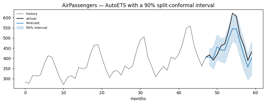
5. Check the coverage

An interval is only worth as much as its coverage. evaluate rolls the fitted object over held-out windows and reports what fraction of actuals landed inside. One window of 12 steps is too small to measure anything, so roll over the last four years instead: four windows of 12 months, each predicted from the history that precedes it.

N_HOLDOUT = 4

histories, truths = [], []
for k in range(N_HOLDOUT):
    end = panel.shape[1] - (N_HOLDOUT - k) * HORIZON
    histories.append(panel[:, :end])
    truths.append(panel[:, end : end + HORIZON])

report = evaluate(fitted, histories, np.stack(truths, axis=1))

print(f"target coverage   {1 - report.alpha:.0%}")
print(f"measured coverage {report.marginal_coverage:.1%}")
print(f"mean width        {report.mean_interval_width:.1f} passengers")

target coverage   90%
measured coverage 93.8%
mean width        128.2 passengers

Marginal is not conditional Conformal coverage is a guarantee on average over draws, not a promise about any one cell. Coverage averaged over series and horizons can sit at 90% while a particular horizon step is systematically under-covered — which is exactly what coverage_by_horizon and coverage_by_series are for. AirPassengers also has a strong upward trend, so the exchangeability that split conformal assumes is only approximately true here; the adaptive methods exist for precisely that reason.

print(report.summary())

Report — SplitConformal
  target coverage: 0.900
  marginal coverage: 0.938
  coverage by horizon: [1.000, 1.000, 1.000, 1.000, 1.000, 1.000, 0.500, 0.750, 1.000, 1.000, 1.000, 1.000]
  mean width: 128.190
  mean Winkler score: 149.198
  n_holdout_samples: 4

The per-horizon breakdown makes the point concretely: the marginal figure is comfortably above target, but step 7 — the summer peak, where a trending series is hardest to bound — covered only half its windows. A single number would have hidden that.

Methods — the six methods, what each one is for, and when split conformal is not enough.
Diagnostics — measuring an interval properly.
Adapters — mlforecast, neuralforecast, or your own model.
Architecture — the method as configuration, and the fitted object it returns.

Getting Started

Concepts

Capabilities

Methods

Nixtlaverse

API Reference

1. The data

2. Fit a forecaster and wrap it

3. Calibrate

4. Predict

5. Check the coverage

Next

​1. The data

​2. Fit a forecaster and wrap it

​3. Calibrate

​4. Predict

​5. Check the coverage

​Next

1. The data

2. Fit a forecaster and wrap it

3. Calibrate

4. Predict

5. Check the coverage

Next