Exogenous features

Your forecaster keeps its own features. X is a separate block handed to the calibration, letting interval width vary with the step being predicted rather than resting only on the size of recent errors. This page threads a feature block through calibration and prediction, and shows what SPCI does with it.

The shape

X is 4-D: (n_series, n_windows | n_samples, horizon, n_features). One feature vector per predicted step, not per observation. If you are forecasting 12 months ahead with 3 features, the last two axes are (12, 3): the features that describe each of those twelve future months.

What is supported in v0.1 Exogenous support is narrower than the array shape suggests:

calibrate_cv(X=...) always raises NotImplementedError. Cross-validated calibration with exogenous features is not implemented. Use the explicit calibrate(forecaster, histories, truths, X=...) loop, which is what this page does.

CQR rejects X entirely — both calibrate(X=...) and predict(X=...) raise, because the quantile path has nowhere to put it.

All three Nixtla adapters carry X through predict, given a train_df holding the regressors’ history. StatsForecast and MLForecast opt in with exog_features=[...]; NeuralForecast reads the list off the model’s futr_exog_list, since a model built that way requires those values. But that is the forecaster using its own features, which is a different thing from the calibration seeing X. It is not a lesser thing: a model that reads its regressors makes sharper point forecasts, which shrinks the calibration residuals and so the interval, for every method. What it does not give you is width that varies with the step being predicted.

refit and quantile methods are unavailable on an exogenous adapter. A history panel is target-only, so a refit would drop the regressors, and predict_quantiles has no X in its contract to feed them.

SPCI reads X at calibrate time, not at predict time. Its interval() ignores the X you pass and queries with the most recent calibration row instead, so future features shape the regressors it fits, not the query it answers.

So feeding X to the calibration still means CallableAdapter. That is what the rest of this page uses.

Features from the calendar

AirPassengers carries no exogenous variables, so build them from its own index: a trend and two Fourier pairs for the yearly cycle. These are known in advance, which is what makes them legitimate: at prediction time you can state the features of a month that has not happened yet.

import matplotlib.pyplot as plt
import numpy as np
import pandas as pd
from sklearn.linear_model import Ridge

from conformalforecast import SequentialPredictiveConformalInference, SplitConformal
from conformalforecast.adapters import CallableAdapter

HORIZON, SEASON, ALPHA = 6, 12, 0.1

df = pd.read_csv("nbs/data/air_passengers.csv", parse_dates=["ds"])
series = df["y"].to_numpy()
T = series.size


def features_at(times):
    """Trend plus two Fourier pairs, for any set of absolute time indices."""
    times = np.asarray(times, dtype=float)
    angle = 2 * np.pi * times / SEASON
    return np.column_stack(
        [
            times / T,
            np.sin(angle),
            np.cos(angle),
            np.sin(2 * angle),
            np.cos(2 * angle),
        ]
    )


N_FEATURES = features_at([0]).shape[1]
print(f"{N_FEATURES} features per predicted step")

5 features per predicted step

A forecaster that takes `X`

CallableAdapter wraps any function of the history. If the function declares an X keyword, the adapter forwards the exogenous block to it; if it does not, X is ignored. That is the whole contract.

def ridge_forecast(history, X=None):
    """Fit a ridge on (features -> y) over the history, predict the next steps.

    history : (n_series, t)      observations so far, NaN-padded on the left
    X       : (n_series, 1, horizon, n_features) features for the steps to predict
    returns : (n_series, horizon)
    """
    n_series, t = history.shape
    out = np.empty((n_series, HORIZON))
    for s in range(n_series):
        observed = ~np.isnan(history[s])
        times = np.flatnonzero(observed)
        model = Ridge(alpha=1.0).fit(features_at(times), history[s, times])
        future = features_at(np.arange(t, t + HORIZON)) if X is None else X[s, 0]
        out[s] = model.predict(future)
    return out


forecaster = CallableAdapter(predict_fn=ridge_forecast, horizon=HORIZON, n_series=1)

Calibrating with `X`

The explicit loop needs three aligned things: a list of histories, the truths that followed each one, and the features of those truths’ timestamps.

N_CALIBRATION, N_HOLDOUT = 60, 4
# The last N_HOLDOUT * HORIZON months are the holdout, so the newest
# calibration window has to stop where that block starts.
HOLDOUT_START = T - N_HOLDOUT * HORIZON

histories, truths, exog = [], [], []
for k in range(N_CALIBRATION, 0, -1):
    end = HOLDOUT_START - HORIZON - k + 1
    histories.append(series[None, :end])
    truths.append(series[None, end : end + HORIZON])
    exog.append(features_at(np.arange(end, end + HORIZON))[None])

truths = np.stack(truths, axis=1)
X_calibration = np.stack(exog, axis=1)

print("histories   ", len(histories), "each (1, t)")
print("truths      ", truths.shape, "(n_series, n_windows, horizon)")
print("X           ", X_calibration.shape, "(n_series, n_windows, horizon, n_features)")

histories    60 each (1, t)
truths       (1, 60, 6) (n_series, n_windows, horizon)
X            (1, 60, 6, 5) (n_series, n_windows, horizon, n_features)

spci_method = SequentialPredictiveConformalInference(alpha=ALPHA, window_size=24, refit_every=4)
spci = spci_method.calibrate(forecaster, histories, truths, X=X_calibration)

split = SplitConformal(alpha=ALPHA).calibrate(forecaster, histories, truths)

print("calibrated on", spci.n_calibration_samples_, "windows")

calibrated on [60] windows

SPCI folds X into the feature vector of each cell’s quantile regressor, alongside the previous window_size residuals. So the width it predicts for a step can depend on which step it is — which month of the year, how far into the trend — and not only on how large the recent errors were. That happens at fit time. The fitted object’s interval() discards the X handed to it and queries with the most recent calibration row, so the “with X” numbers below differ through the regressors it fitted and the point forecast it was given — not through an interval query conditioned on the future features. Split conformal ignores X even when given it: its score is a plain absolute residual with nowhere to put a feature. Passing X to a method that cannot use it is not an error, and not useful either.

Predicting with `X`

At prediction time the features describe the steps you are about to forecast.

end = T - HORIZON
X_future = features_at(np.arange(end, end + HORIZON))[None, None]
print("X_future", X_future.shape)

spci_prediction = spci.predict(series[None, :end], X=X_future)
split_prediction = split.predict(series[None, :end])

steps = np.arange(1, HORIZON + 1)
fig, ax = plt.subplots(figsize=(9, 3.8))
ax.plot(steps, series[end:], color="k", lw=1.6, label="actual")
ax.plot(steps, spci_prediction.point[0, 0], color="C0", lw=1.3, ls=":", label="ridge forecast")
ax.fill_between(
    steps,
    spci_prediction.interval[0, 0, :, 0],
    spci_prediction.interval[0, 0, :, 1],
    color="C0",
    alpha=0.25,
    label="SPCI with X",
)
ax.plot(
    steps,
    split_prediction.interval[0, 0, :, 0],
    color="0.45",
    lw=1.2,
    ls="--",
    label="split conformal (no X)",
)
ax.plot(steps, split_prediction.interval[0, 0, :, 1], color="0.45", lw=1.2, ls="--")
ax.set_xlabel("horizon (months ahead)")
ax.set_ylabel("passengers")
ax.set_title("An X-aware interval against a flat one")
ax.legend(fontsize=8, frameon=False)
fig.tight_layout()

X_future (1, 1, 6, 5)

for name, prediction in [("SPCI with X", spci_prediction), ("split conformal", split_prediction)]:
    width = prediction.interval[0, 0, :, 1] - prediction.interval[0, 0, :, 0]
    print(f"{name:18s} width by step {np.round(width, 1)}")

SPCI with X        width by step [49.  53.4 52.7 38.3 63.2 54.6]
split conformal    width by step [165.1 177.5 183.4 184.8 186.3 189.7]

What the method actually gains

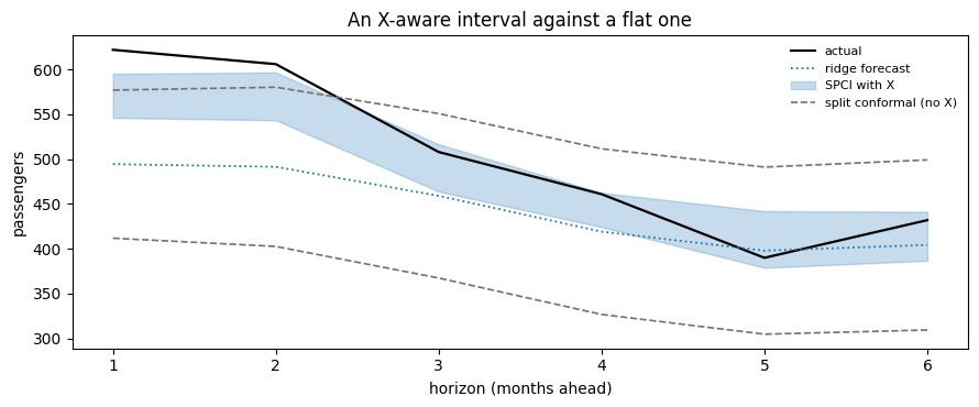
Held out over the last two years, with and without the feature block.

evaluate does not thread X diagnostics.evaluate takes (fitted, histories, truths) and no exogenous argument, so an X-aware holdout has to be rolled by hand. It is six lines, and it also makes the predict / update order explicit — which is worth seeing once.

def roll(fitted, histories, truths, X=None):
    """Predict each holdout window, update online methods, return the intervals."""
    intervals = []
    for k, history in enumerate(histories):
        step_X = None if X is None else X[:, k : k + 1]
        prediction = (
            fitted.predict(history, X=step_X) if step_X is not None else fitted.predict(history)
        )
        intervals.append(prediction.interval[:, 0])
        if fitted.method_.IS_ONLINE:
            truth = truths[:, k : k + 1]
            if step_X is not None:
                fitted.update(prediction.point, truth, X=step_X)
            else:
                fitted.update(prediction.point, truth)
    return np.stack(intervals, axis=1)  # (n_series, n_windows, horizon, 2)


holdout_histories, holdout_truths, holdout_exog = [], [], []
for k in range(N_HOLDOUT, 0, -1):
    end = T - k * HORIZON
    holdout_histories.append(series[None, :end])
    holdout_truths.append(series[None, end : end + HORIZON])
    holdout_exog.append(features_at(np.arange(end, end + HORIZON))[None])
holdout_truths = np.stack(holdout_truths, axis=1)
X_holdout = np.stack(holdout_exog, axis=1)

# The same method config, fitted a second time without X: a separate object.
blind = spci_method.calibrate(forecaster, histories, truths)

for name, fitted, X in [
    ("SPCI with X", spci, X_holdout),
    ("SPCI without X", blind, None),
    ("split conformal", split, None),
]:
    intervals = roll(fitted, holdout_histories, holdout_truths, X)
    covered = (holdout_truths >= intervals[..., 0]) & (holdout_truths <= intervals[..., 1])
    width = intervals[..., 1] - intervals[..., 0]
    print(f"{name:18s} coverage {covered.mean():6.1%}   mean width {width.mean():7.1f}")

SPCI with X        coverage  58.3%   mean width    61.3
SPCI without X     coverage  62.5%   mean width    55.2
split conformal    coverage  83.3%   mean width   181.1

On this problem, the features do not earn their place. SPCI with X is wider than SPCI without it (61.3 against 55.2) and covers worse (58.3% against 62.5%), and both sit far under the 90% target while plain split conformal — which cannot read X at all — covers best at 83.3%. That is a real result, not a broken example, and it has two causes worth separating:

The features are redundant. A trend and two Fourier pairs describe where in the year each step falls. SPCI’s residual window already carries that information implicitly, because the last 24 residuals of a seasonal series encode the season. Giving a model a feature it can already infer adds variance, not signal. Exogenous features pay off when they carry information the residual history cannot contain — a scheduled promotion, a known outage, a holiday calendar that does not repeat annually.
The horizon. SPCI under-covers at multi-step horizons on real series; see the warning on the SPCI page for the measurement and the reason. Both SPCI columns inherit that, with or without X.

The transferable lesson is the one this page opened with: thread the features, then measure. X is a hypothesis about what drives your uncertainty, and diagnostics is how you find out whether it was right.

SPCI — the method that consumes X, in full.
Adapters — writing your own, including the X keyword.
Diagnostics — measuring whether the features earned their place.

Getting Started

Concepts

Capabilities

Methods

Nixtlaverse

API Reference

Exogenous features

The shape

Features from the calendar

A forecaster that takes `X`

Calibrating with `X`

Predicting with `X`

What the method actually gains

Next

​The shape

​Features from the calendar

​A forecaster that takes X

​Calibrating with X

​Predicting with X

​What the method actually gains

​Next

The shape

Features from the calendar

A forecaster that takes `X`

Calibrating with `X`

Predicting with `X`

What the method actually gains

Next