

1. Load and Prepare Data
We use the Australian Tourism dataset for this example.| Country | Region | State | Purpose | ds | y | |
|---|---|---|---|---|---|---|
| 0 | Australia | Adelaide | South Australia | Business | 1998-01-01 | 135.077690 |
| 1 | Australia | Adelaide | South Australia | Business | 1998-04-01 | 109.987316 |
| 2 | Australia | Adelaide | South Australia | Business | 1998-07-01 | 166.034687 |
| 3 | Australia | Adelaide | South Australia | Business | 1998-10-01 | 127.160464 |
| 4 | Australia | Adelaide | South Australia | Business | 1999-01-01 | 137.448533 |
2. Compute Base Forecasts
3. Probabilistic Reconciliation Methods
Method Comparison Table
| Method | Distributional Assumptions | Residual Usage | Reconciliation Timing | Coverage Guarantee | Hierarchy Requirement |
|---|---|---|---|---|---|
| Normality | Gaussian errors | Computes covariance from residuals | N/A (analytical) | Asymptotic | Any |
| Bootstrap | None | Block resamples raw residuals, then reconciles | After perturbation | Asymptotic | Any |
| PERMBU | None (uses empirical marginals) | Rank permutations for copula | Bottom-up aggregation | Asymptotic | Strictly hierarchical only |
| Conformal | Exchangeability | Scores from reconciled residuals | Before perturbation | Finite-sample: | Any |
Key Technical Differences
Bootstrap vs Conformal residual handling: - Bootstrap: Adds residual blocks to raw forecasts, then applies reconciliation (SP @ (y_hat + residuals)) - Conformal: Computes scores from
reconciled forecasts, adds to reconciled predictions
(y_rec + scores)
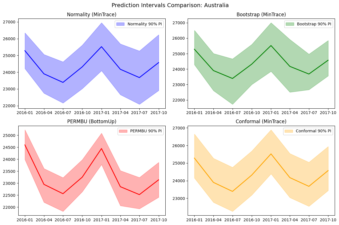
4. Visualize Prediction Intervals
5. Evaluate Probabilistic Forecasts
We evaluate the probabilistic forecasts using the Scaled Continuous Ranked Probability Score (CRPS), which measures the quality of probabilistic predictions. Lower values indicate better calibrated prediction intervals.| level | metric | Normality | Bootstrap | PERMBU | Conformal | |
|---|---|---|---|---|---|---|
| 0 | Country | scaled_crps | 0.027256 | 0.028403 | 0.086038 | 0.028478 |
| 1 | State | scaled_crps | 0.033189 | 0.031690 | 0.065403 | 0.031761 |
| 2 | Region | scaled_crps | 0.046120 | 0.050435 | 0.055291 | 0.049632 |
| 3 | Overall | scaled_crps | 0.044681 | 0.048412 | 0.056605 | 0.047701 |
6. Method Pros and Cons
Normality
Pros: - Fast computation using closed-form solutions - Well-understood theoretical properties - Works with any reconciliation method and hierarchy structure - Supports different covariance estimators (ols, wls_var, mint_shrink, etc.)
Cons: - Assumes Gaussian distribution of errors - May underestimate
uncertainty for heavy-tailed or skewed distributions - Covariance
estimation can be unstable with limited data
Bootstrap
Pros: - Non-parametric: no distributional assumptions required - Captures empirical error distribution shape (skewness, heavy tails) - Preserves temporal correlation through block resampling - Works with any hierarchy structure Cons: - Requires sufficient historical residuals (at least horizon + some buffer) - Computationally more expensive than Normality - Coverage is asymptotic (no finite-sample guarantees)PERMBU
Pros: - Preserves empirical dependencies using copula-based approach - Respects marginal distributions at each level - Captures complex cross-series dependencies Cons: - Only works with strictly hierarchical structures (not grouped hierarchies) - Computationally intensive for large hierarchies - Requires careful handling of the permutation orderingConformal
Pros: - Distribution-free: no parametric assumptions required - Finite-sample coverage guarantee under exchangeability - Simple interpretation: intervals based on empirical quantiles of scores - Works with any hierarchy structure Cons: - Requires proper calibration set: Coverage guarantees assume the calibration data is independent from training data. When using in-sample residuals (fitted values from the same data used to train the model), this assumption is violated, potentially leading to overly optimistic (narrow) intervals - Exchangeability assumption may not hold for time series with trends or structural breaks - Coverage guarantees are marginal (per-series), not simultaneous across the hierarchy - May produce wider intervals than well-specified parametric methods ⚠️ Important Caveat for Conformal: In this example (and the default HierarchicalForecast API), we use in-sample fitted values as the calibration set. This is convenient but technically violates the split conformal prediction framework. For rigorous coverage guarantees, you should use a held-out validation set that was not used for model training.7. Recommendations
| Scenario | Recommended Method | Notes |
|---|---|---|
| Quick analysis, errors appear Gaussian | Normality | Fastest, well-understood |
| Unknown error distribution, general use | Bootstrap | Safe default, no assumptions |
| Strict hierarchies, need correlation preservation | PERMBU | Best for capturing dependencies |
| Have proper held-out calibration set | Conformal | Valid finite-sample guarantees |
| Using in-sample residuals, want simplicity | Bootstrap or Normality | Conformal caveats apply with in-sample data |
Decision Flowchart
- Is your hierarchy strictly hierarchical (no
cross-classifications)?
- Yes → Consider PERMBU if you need correlation preservation
- No → Use Normality, Bootstrap, or Conformal
- Do you have a proper held-out calibration set?
- Yes → Conformal provides finite-sample coverage guarantees
- No (using in-sample) → Bootstrap or Normality are more appropriate
- Do your residuals appear Gaussian?
- Yes → Normality is fast and efficient
- No / Unknown → Bootstrap adapts to any distribution