Normality

In many cases, only the time series at the lowest level of the hierarchies (bottom time series) are available. HierarchicalForecast has tools to create time series for all hierarchies and also allows you to calculate prediction intervals for all hierarchies. In this notebook we will see how to do it.

!pip install hierarchicalforecast statsforecast

import numpy as np
import pandas as pd
import matplotlib.pyplot as plt

# compute base forecast no coherent
from statsforecast.models import AutoARIMA
from statsforecast.core import StatsForecast

#obtain hierarchical reconciliation methods and evaluation
from hierarchicalforecast.methods import BottomUp, MinTrace
from hierarchicalforecast.utils import aggregate, HierarchicalPlot
from hierarchicalforecast.core import HierarchicalReconciliation
from hierarchicalforecast.evaluation import HierarchicalEvaluation

/Users/fedex/miniconda3/envs/hierarchicalforecast/lib/python3.10/site-packages/statsforecast/core.py:21: TqdmWarning: IProgress not found. Please update jupyter and ipywidgets. See https://ipywidgets.readthedocs.io/en/stable/user_install.html
  from tqdm.autonotebook import tqdm

Aggregate bottom time series

In this example we will use the Tourism dataset from the Forecasting: Principles and Practice book. The dataset only contains the time series at the lowest level, so we need to create the time series for all hierarchies.

Y_df = pd.read_csv('https://raw.githubusercontent.com/Nixtla/transfer-learning-time-series/main/datasets/tourism.csv')
Y_df = Y_df.rename({'Trips': 'y', 'Quarter': 'ds'}, axis=1)
Y_df.insert(0, 'Country', 'Australia')
Y_df = Y_df[['Country', 'Region', 'State', 'Purpose', 'ds', 'y']]
Y_df['ds'] = Y_df['ds'].str.replace(r'(\d+) (Q\d)', r'\1-\2', regex=True)
Y_df['ds'] = pd.to_datetime(Y_df['ds'])
Y_df.head()

	Country	Region	State	Purpose	ds	y
0	Australia	Adelaide	South Australia	Business	1998-01-01	135.077690
1	Australia	Adelaide	South Australia	Business	1998-04-01	109.987316
2	Australia	Adelaide	South Australia	Business	1998-07-01	166.034687
3	Australia	Adelaide	South Australia	Business	1998-10-01	127.160464
4	Australia	Adelaide	South Australia	Business	1999-01-01	137.448533

The dataset can be grouped in the following non-strictly hierarchical structure.

spec = [
    ['Country'],
    ['Country', 'State'], 
    ['Country', 'Purpose'], 
    ['Country', 'State', 'Region'], 
    ['Country', 'State', 'Purpose'], 
    ['Country', 'State', 'Region', 'Purpose']
]

Using the aggregate function from HierarchicalForecast we can generate: 1. Y_df: the hierarchical structured series $\mathbf{y}_{[a,b]\tau}$ 2. S_df: the aggregation constraings dataframe with $S_{[a,b]}$ 3. tags: a list with the ‘unique_ids’ conforming each aggregation level.

Y_df, S_df, tags = aggregate(df=Y_df, spec=spec)
Y_df = Y_df.reset_index()

/Users/fedex/miniconda3/envs/hierarchicalforecast/lib/python3.10/site-packages/sklearn/preprocessing/_encoders.py:828: FutureWarning: `sparse` was renamed to `sparse_output` in version 1.2 and will be removed in 1.4. `sparse_output` is ignored unless you leave `sparse` to its default value.
  warnings.warn(

Y_df.head()

	unique_id	ds	y
0	Australia	1998-01-01	23182.197269
1	Australia	1998-04-01	20323.380067
2	Australia	1998-07-01	19826.640511
3	Australia	1998-10-01	20830.129891
4	Australia	1999-01-01	22087.353380

S_df.iloc[:5, :5]

	Australia/ACT/Canberra/Business	Australia/ACT/Canberra/Holiday	Australia/ACT/Canberra/Other	Australia/ACT/Canberra/Visiting	Australia/New South Wales/Blue Mountains/Business
Australia	1.0	1.0	1.0	1.0	1.0
Australia/ACT	1.0	1.0	1.0	1.0	0.0
Australia/New South Wales	0.0	0.0	0.0	0.0	1.0
Australia/Northern Territory	0.0	0.0	0.0	0.0	0.0
Australia/Queensland	0.0	0.0	0.0	0.0	0.0

tags['Country/Purpose']

array(['Australia/Business', 'Australia/Holiday', 'Australia/Other',
       'Australia/Visiting'], dtype=object)

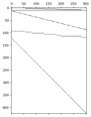
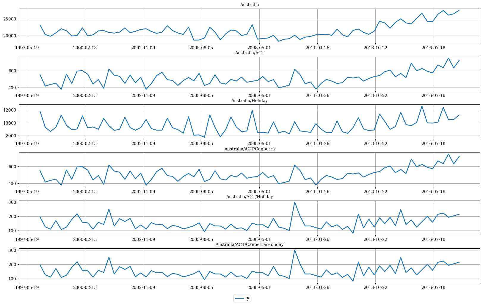
We can visualize the S matrix and the data using the HierarchicalPlot class as follows.

hplot = HierarchicalPlot(S=S_df, tags=tags)

hplot.plot_summing_matrix()

hplot.plot_hierarchically_linked_series(
    bottom_series='Australia/ACT/Canberra/Holiday',
    Y_df=Y_df.set_index('unique_id')
)

Split Train/Test sets

We use the final two years (8 quarters) as test set.

Y_test_df = Y_df.groupby('unique_id').tail(8)
Y_train_df = Y_df.drop(Y_test_df.index)

Y_test_df = Y_test_df.set_index('unique_id')
Y_train_df = Y_train_df.set_index('unique_id')

Y_train_df.groupby('unique_id').size()

unique_id
Australia                                                72
Australia/ACT                                            72
Australia/ACT/Business                                   72
Australia/ACT/Canberra                                   72
Australia/ACT/Canberra/Business                          72
                                                         ..
Australia/Western Australia/Experience Perth/Other       72
Australia/Western Australia/Experience Perth/Visiting    72
Australia/Western Australia/Holiday                      72
Australia/Western Australia/Other                        72
Australia/Western Australia/Visiting                     72
Length: 425, dtype: int64

Computing base forecasts

The following cell computes the base forecasts for each time series in Y_df using the AutoARIMA and model. Observe that Y_hat_df contains the forecasts but they are not coherent. To reconcile the prediction intervals we need to calculate the uncoherent intervals using the level argument of StatsForecast.

fcst = StatsForecast(df=Y_train_df,
                     models=[AutoARIMA(season_length=4)], 
                     freq='QS', n_jobs=-1)
Y_hat_df = fcst.forecast(h=8, fitted=True, level=[80, 90])
Y_fitted_df = fcst.forecast_fitted_values()

Reconcile forecasts

The following cell makes the previous forecasts coherent using the HierarchicalReconciliation class. Since the hierarchy structure is not strict, we can’t use methods such as TopDown or MiddleOut. In this example we use BottomUp and MinTrace. If you want to calculate prediction intervals, you have to use the level argument as follows.

reconcilers = [
    BottomUp(),
    MinTrace(method='mint_shrink'),
    MinTrace(method='ols')
]
hrec = HierarchicalReconciliation(reconcilers=reconcilers)
Y_rec_df = hrec.reconcile(Y_hat_df=Y_hat_df, Y_df=Y_fitted_df, 
                          S=S_df, tags=tags, level=[80, 90])

The dataframe Y_rec_df contains the reconciled forecasts.

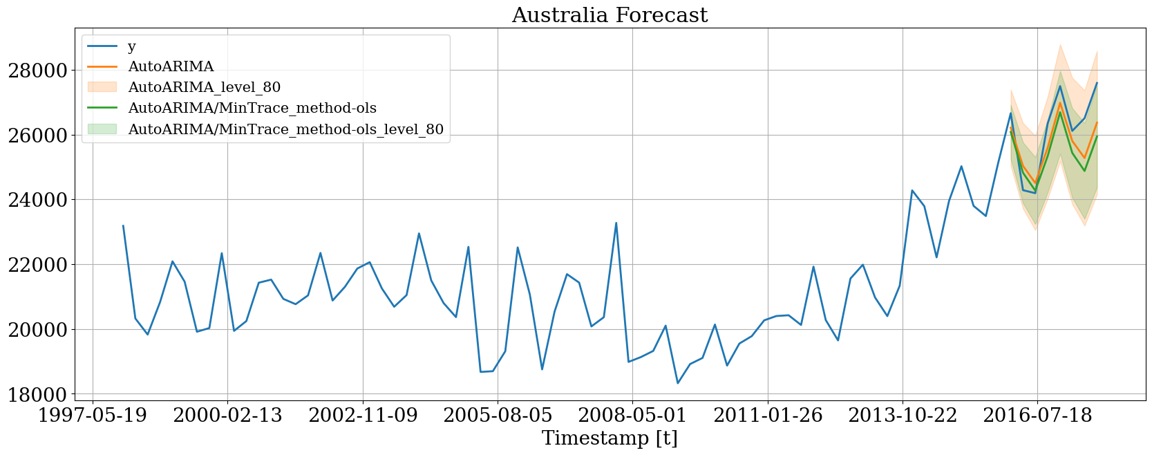
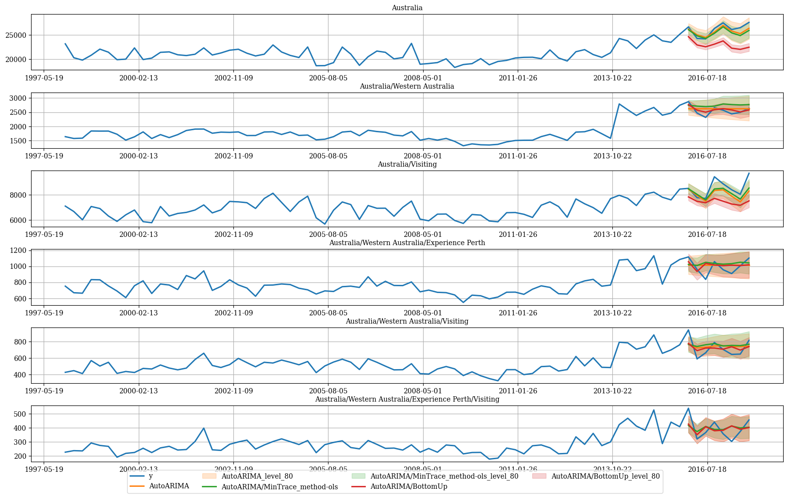
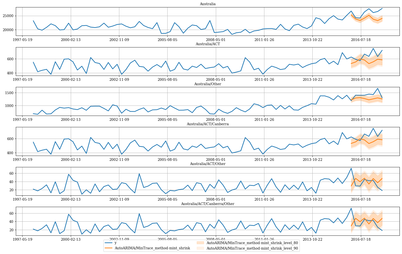
Y_rec_df.head()

	ds	AutoARIMA	AutoARIMA-lo-90	AutoARIMA-lo-80	AutoARIMA-hi-80	AutoARIMA-hi-90	AutoARIMA/BottomUp	AutoARIMA/BottomUp-lo-90	AutoARIMA/BottomUp-lo-80	AutoARIMA/BottomUp-hi-80	…	AutoARIMA/MinTrace_method-mint_shrink	AutoARIMA/MinTrace_method-mint_shrink-lo-90	AutoARIMA/MinTrace_method-mint_shrink-lo-80	AutoARIMA/MinTrace_method-mint_shrink-hi-80	AutoARIMA/MinTrace_method-mint_shrink-hi-90	AutoARIMA/MinTrace_method-ols	AutoARIMA/MinTrace_method-ols-lo-90	AutoARIMA/MinTrace_method-ols-lo-80	AutoARIMA/MinTrace_method-ols-hi-80	AutoARIMA/MinTrace_method-ols-hi-90
unique_id
Australia	2016-01-01	26212.554688	24694.224609	25029.580078	27395.527344	27730.884766	24368.099609	23674.076441	23827.366706	24908.832513	…	25205.749397	24453.417115	24619.586229	25791.912565	25958.081679	26059.047512	24978.608364	25217.247087	26900.847937	27139.486661
Australia	2016-04-01	25033.667969	23324.066406	23701.669922	26365.666016	26743.269531	22395.921875	21629.482078	21798.767146	22993.076604	…	23720.833190	22915.772233	23093.587632	24348.078748	24525.894148	24769.464257	23554.946551	23823.199470	25715.729045	25983.981963
Australia	2016-07-01	24507.027344	22625.500000	23041.076172	25972.978516	26388.554688	22004.169922	21182.945074	21364.330624	22644.009219	…	23167.123691	22316.298074	22504.221604	23830.025777	24017.949308	24205.855344	22870.661086	23165.568073	25246.142616	25541.049603
Australia	2016-10-01	25598.929688	23559.919922	24010.281250	27187.578125	27637.937500	22325.056641	21456.892977	21648.645996	23001.467285	…	23982.251913	23087.313715	23284.980478	24679.523348	24877.190111	25271.861336	23825.782311	24145.180634	26398.542038	26717.940362
Australia	2017-01-01	26982.578125	24651.535156	25166.396484	28798.757812	29313.619141	23258.001953	22296.178714	22508.618508	24007.385398	…	25002.243615	24016.747195	24234.415731	25770.071498	25987.740034	26611.143736	24959.636647	25324.408272	27897.879201	28262.650825

Plot forecasts

Then we can plot the probabilistic forecasts using the following function.

plot_df = pd.concat([Y_df.set_index(['unique_id', 'ds']), 
                     Y_rec_df.set_index('ds', append=True)], axis=1)
plot_df = plot_df.reset_index('ds')

Plot single time series

hplot.plot_series(
    series='Australia',
    Y_df=plot_df, 
    models=['y', 'AutoARIMA', 'AutoARIMA/MinTrace_method-ols'],
    level=[80]
)

# Since we are plotting a bottom time series
# the probabilistic and mean forecasts
# are the same
hplot.plot_series(
    series='Australia/Western Australia/Experience Perth/Visiting',
    Y_df=plot_df, 
    models=['y', 'AutoARIMA', 'AutoARIMA/BottomUp'],
    level=[80]
)

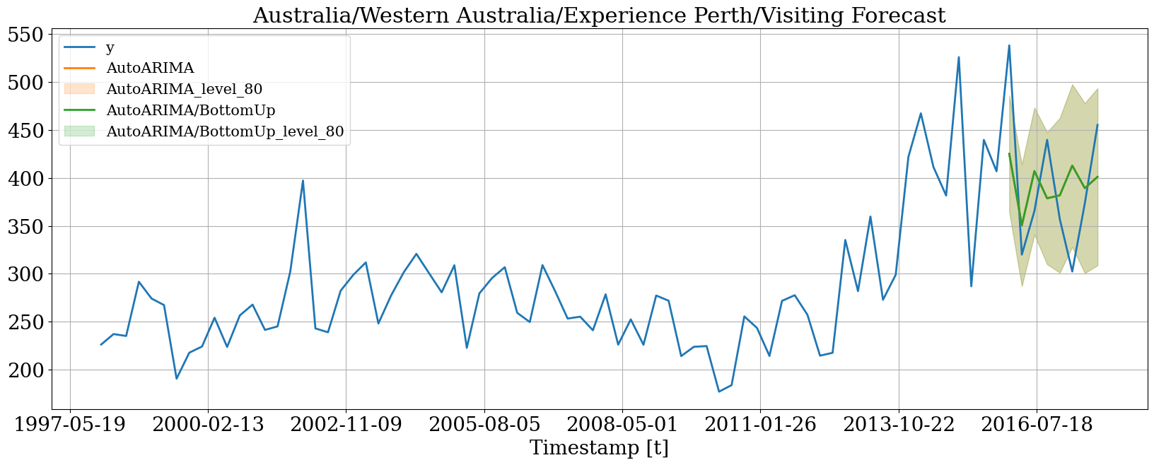
Plot hierarchichally linked time series

hplot.plot_hierarchically_linked_series(
    bottom_series='Australia/Western Australia/Experience Perth/Visiting',
    Y_df=plot_df, 
    models=['y', 'AutoARIMA', 'AutoARIMA/MinTrace_method-ols', 'AutoARIMA/BottomUp'],
    level=[80]
)

# ACT only has Canberra
hplot.plot_hierarchically_linked_series(
    bottom_series='Australia/ACT/Canberra/Other',
    Y_df=plot_df, 
    models=['y', 'AutoARIMA/MinTrace_method-mint_shrink'],
    level=[80, 90]
)

Getting Started

Tutorials

API Reference

Aggregate bottom time series

Split Train/Test sets

Computing base forecasts

Reconcile forecasts

Plot forecasts

Plot single time series

Plot hierarchichally linked time series

References

Getting Started

Tutorials

API Reference

​Aggregate bottom time series

​Split Train/Test sets

​Computing base forecasts

​Reconcile forecasts

​Plot forecasts

​Plot single time series

​Plot hierarchichally linked time series

​References

Aggregate bottom time series

Split Train/Test sets

Computing base forecasts

Reconcile forecasts

Plot forecasts

Plot single time series

Plot hierarchichally linked time series

References