This example notebook demonstrates the compatibility of HierarchicalForecast’s reconciliation methods with popular machine-learning libraries, specifically NeuralForecast and MLForecast.

The notebook utilizes NBEATS and XGBRegressor models to create base forecasts for the TourismLarge Hierarchical Dataset. After that, we use HierarchicalForecast to reconcile the base predictions.

References
- Boris N. Oreshkin, Dmitri Carpov, Nicolas Chapados, Yoshua Bengio (2019). “N-BEATS: Neural basis expansion analysis for interpretable time series forecasting”. url: https://arxiv.org/abs/1905.10437
- Tianqi Chen and Carlos Guestrin. “XGBoost: A Scalable Tree Boosting System”. In: Proceedings of the 22nd ACM SIGKDD International Conference on Knowledge Discovery and Data Mining. KDD ’16. San Francisco, California, USA: Association for Computing Machinery, 2016, pp. 785–794. isbn: 9781450342322. doi: 10.1145/2939672.2939785. url: https://doi.org/10.1145/2939672.2939785 (cit. on p. 26).

You can run these experiments using CPU or GPU with Google Colab.

Open In Colab

1. Installing packages

# %pip install datasetsforecast hierarchicalforecast mlforecast neuralforecast
import numpy as np
import pandas as pd

from datasetsforecast.hierarchical import HierarchicalData

from neuralforecast import NeuralForecast
from neuralforecast.models import NBEATS
from neuralforecast.losses.pytorch import GMM

from mlforecast import MLForecast
from mlforecast.utils import PredictionIntervals
import xgboost as xgb

#obtain hierarchical reconciliation methods and evaluation
from hierarchicalforecast.methods import BottomUp, ERM, MinTrace
from hierarchicalforecast.utils import HierarchicalPlot
from hierarchicalforecast.core import HierarchicalReconciliation
from hierarchicalforecast.evaluation import scaled_crps

2. Load hierarchical dataset

This detailed Australian Tourism Dataset comes from the National Visitor Survey, managed by the Tourism Research Australia, it is composed of 555 monthly series from 1998 to 2016, it is organized geographically, and purpose of travel. The natural geographical hierarchy comprises seven states, divided further in 27 zones and 76 regions. The purpose of travel categories are holiday, visiting friends and relatives (VFR), business and other. The MinT (Wickramasuriya et al., 2019), among other hierarchical forecasting studies has used the dataset it in the past. The dataset can be accessed in the MinT reconciliation webpage, although other sources are available.

Geographical DivisionNumber of series per divisionNumber of series per purposeTotal
Australia145
States72835
Zones27108135
Regions76304380
Total111444555
Y_df, S_df, tags = HierarchicalData.load('./data', 'TourismLarge')
Y_df['ds'] = pd.to_datetime(Y_df['ds'])
Y_df.head()
unique_iddsy
0TotalAll1998-01-0145151.071280
1TotalAll1998-02-0117294.699551
2TotalAll1998-03-0120725.114184
3TotalAll1998-04-0125388.612353
4TotalAll1998-05-0120330.035211

Visualize the aggregation matrix.

hplot = HierarchicalPlot(S=S_df, tags=tags)
hplot.plot_summing_matrix()

Split the dataframe in train/test splits.

def sort_hier_df(Y_df, S_df):
    # sorts unique_id lexicographically
    Y_df.unique_id = Y_df.unique_id.astype('category')
    Y_df.unique_id = Y_df.unique_id.cat.set_categories(S_df.index)
    Y_df = Y_df.sort_values(by=['unique_id', 'ds'])
    return Y_df

Y_df = sort_hier_df(Y_df, S_df)
horizon = 12
Y_test_df = Y_df.groupby('unique_id').tail(horizon)
Y_train_df = Y_df.drop(Y_test_df.index)

3. Fit and Predict Models

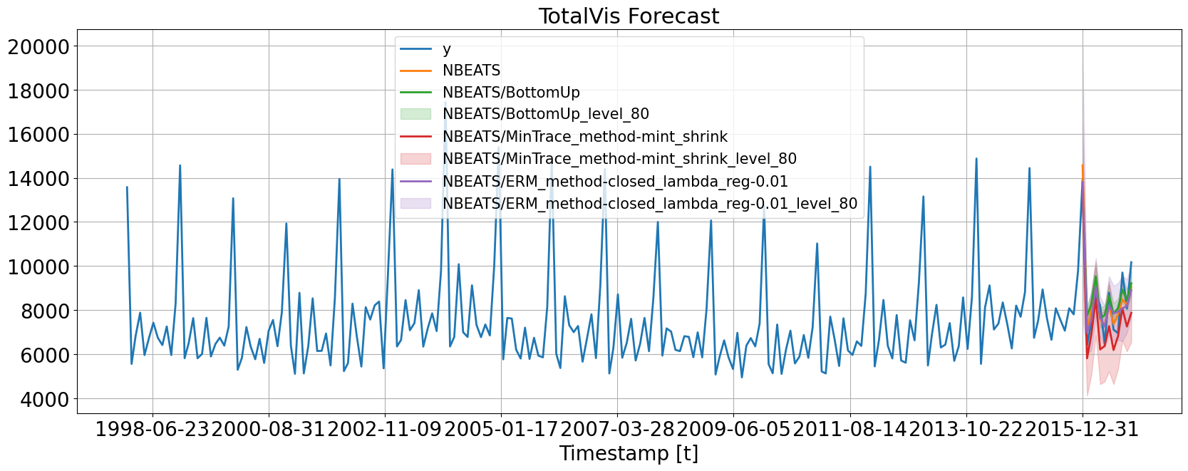
HierarchicalForecast is compatible with many different ML models. Here, we show two examples:
1. NBEATS, a MLP-based deep neural architecture.
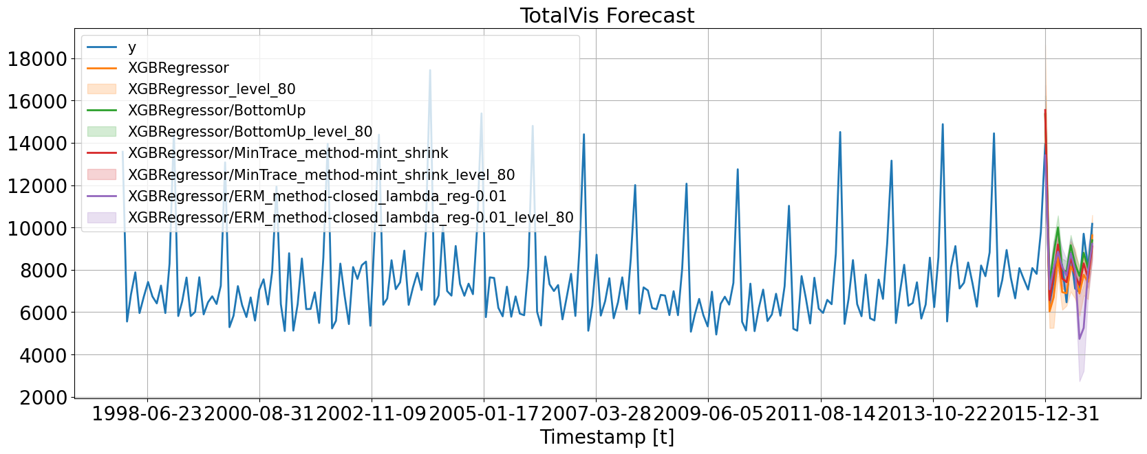
2. XGBRegressor, a tree-based architecture.

level = np.arange(0, 100, 2)
qs = [[50-lv/2, 50+lv/2] for lv in level]
quantiles = np.sort(np.concatenate(qs)/100)

#fit/predict NBEATS from NeuralForecast
nbeats = NBEATS(h=horizon,
              input_size=2*horizon,
              loss=GMM(n_components=10, quantiles=quantiles),
              scaler_type='robust',
              max_steps=2000)
nf = NeuralForecast(models=[nbeats], freq='MS')
nf.fit(df=Y_train_df)
Y_hat_nf = nf.predict()
insample_nf = nf.predict_insample(step_size=horizon)

#fit/predict XGBRegressor from MLForecast
mf = MLForecast(models=[xgb.XGBRegressor()], 
                freq='MS',
                lags=[1,2,12,24],
                date_features=['month'],
                )
mf.fit(Y_train_df, fitted=True, prediction_intervals=PredictionIntervals(n_windows=10, h=horizon)) 
Y_hat_mf = mf.predict(horizon, level=level).set_index('unique_id')
insample_mf = mf.forecast_fitted_values()
Y_hat_nf
dsNBEATSNBEATS-lo-98.0NBEATS-lo-96.0NBEATS-lo-94.0NBEATS-lo-92.0NBEATS-lo-90.0NBEATS-lo-88.0NBEATS-lo-86.0NBEATS-lo-84.0NBEATS-hi-80.0NBEATS-hi-82.0NBEATS-hi-84.0NBEATS-hi-86.0NBEATS-hi-88.0NBEATS-hi-90.0NBEATS-hi-92.0NBEATS-hi-94.0NBEATS-hi-96.0NBEATS-hi-98.0
unique_id
TotalAll2016-01-0144525.65234421232.55468826024.83984427435.28515628136.70507828766.15039129569.24023430344.24023431163.09960951812.95312552171.79296952628.56250052890.75000053160.31250054025.21093854451.10937555651.00781257686.02734461461.066406
TotalAll2016-02-0120819.43164118020.28906218314.94335918480.26953118612.46484418695.38281218807.24218818912.91015619027.18750022719.99804722802.92187522887.73437523031.00585923133.86523423230.32226623406.49609423622.16601623887.79687524165.496094
TotalAll2016-03-0123676.29101619303.22265619684.69335919928.40039120150.69140620319.11328120499.98046920632.18554720748.20703126215.31250026291.19531226402.85351626578.25781226848.17968827054.10742227310.74609427723.86718828211.29492229011.082031
TotalAll2016-04-0127978.58789123936.98828124329.89257824532.74023424735.70312524902.81250025165.07421925256.66992225489.45507830192.36523430278.45117230339.01757830381.44335930465.72265630574.05664130682.60937530860.42773431032.64843831199.992188
TotalAll2016-05-0122810.31054720037.21875020194.53125020387.54101620510.24414120594.22656220675.72070320767.02539120876.55078124975.91601625149.09765625240.17773425401.99609425577.40039125800.57421926132.90429726559.90625027273.56640628567.857422
GBDOth2016-08-013.384338-31.891897-15.230768-1.954657-1.143704-0.994592-0.947800-0.884839-0.8247489.63507410.51704411.37498812.78455614.56841322.58166937.88090551.51248662.64597781.495415
GBDOth2016-09-014.842800-41.682514-23.578377-6.487054-1.238661-1.024779-0.927368-0.856639-0.75856811.74363012.75523014.38478016.57934419.42572636.15553744.39454360.14474978.533859101.363129
GBDOth2016-10-014.466261-21.124041-1.662255-1.157058-0.949211-0.857361-0.755605-0.699540-0.65941910.40519311.60576912.68668714.21890019.96374126.70527334.36116051.89855268.36193189.458908
GBDOth2016-11-013.689114-22.615982-11.813770-1.530864-1.049960-0.922807-0.868391-0.802971-0.7234628.2132608.83767010.21945712.30093213.13582923.32576037.62852543.99338263.59431584.825226
GBDOth2016-12-013.994789-38.856083-24.361221-7.503808-1.199999-1.003695-0.880594-0.788414-0.7374899.88115711.40633412.63697715.83153626.05926932.27000037.31646051.76577468.93330491.916100
Y_hat_mf
dsXGBRegressorXGBRegressor-lo-98XGBRegressor-lo-96XGBRegressor-lo-94XGBRegressor-lo-92XGBRegressor-lo-90XGBRegressor-lo-88XGBRegressor-lo-86XGBRegressor-lo-84XGBRegressor-hi-80XGBRegressor-hi-82XGBRegressor-hi-84XGBRegressor-hi-86XGBRegressor-hi-88XGBRegressor-hi-90XGBRegressor-hi-92XGBRegressor-hi-94XGBRegressor-hi-96XGBRegressor-hi-98
unique_id
TotalAll2016-01-0143060.22656238276.97448338677.67053039078.36657739479.06262439879.75867140009.21887740041.80914040074.39940345980.87319546013.46345946046.05372246078.64398546111.23424846240.69445446641.39050147042.08654847442.78259547843.478642
TotalAll2016-02-0118008.29687514687.96286814813.81646714939.67006615065.52366615191.37726515247.40053915278.48441015309.56828120644.85772620675.94159720707.02546920738.10934020769.19321120825.21648520951.07008421076.92368421202.77728321328.630882
TotalAll2016-03-0120694.08007816407.35109916594.14904316780.94698716967.74493117154.54287517209.43467717217.21714117224.99960624147.59562024155.37808524163.16055024170.94301524178.72548024233.61728124420.41522524607.21316924794.01111324980.809057
TotalAll2016-04-0124474.34960920859.12055820978.73772621098.35489321217.97206021337.58922721380.28716721395.51395321410.74073927507.50490627522.73169327537.95847927553.18526627568.41205227611.10999127730.72715927850.34432627969.96149328089.578660
TotalAll2016-05-0119281.08789115045.23584915460.10899015874.98213116289.85527116704.72841216861.92779616927.10083716992.27387821439.55582221504.72886321569.90190421635.07494521700.24798621857.44736922272.32051022687.19365123102.06679223516.939933
GBDOth2016-08-0111.040442-0.7202640.9348772.5900174.2451575.9002986.3969936.4799576.56292115.35203515.43500015.51796415.60092815.68389216.18058717.83572719.49086821.14600822.801149
GBDOth2016-09-016.440751-0.275863-0.182214-0.0885660.0050830.0987320.1233760.1233760.12337612.75812612.75812612.75812612.75812612.75812612.78277112.87641912.97006813.06371613.157365
GBDOth2016-10-019.9951122.4078702.4078702.4078702.4078702.4078702.4078702.4078702.40787017.58235517.58235517.58235517.58235517.58235517.58235517.58235517.58235517.58235517.582355
GBDOth2016-11-016.7475662.7913892.7913892.7913892.7913892.7913892.7913892.7913892.79138910.70374210.70374210.70374210.70374210.70374210.70374210.70374210.70374210.70374210.703742
GBDOth2016-12-017.3679042.3492002.3492002.3492002.3492002.3492002.3492002.3492002.34920012.38660912.38660912.38660912.38660912.38660912.38660912.38660912.38660912.38660912.386609

4. Reconcile Predictions

With minimal parsing, we can reconcile the raw output predictions with different HierarchicalForecast reconciliation methods.

reconcilers = [
    ERM(method='closed'),
    BottomUp(),
    MinTrace('ols'),
]
hrec = HierarchicalReconciliation(reconcilers=reconcilers)

Y_rec_nf = hrec.reconcile(Y_hat_df=Y_hat_nf, Y_df=insample_nf, S=S_df, tags=tags, level=level)
Y_rec_mf = hrec.reconcile(Y_hat_df=Y_hat_mf, Y_df=insample_mf, S=S_df, tags=tags, level=level)

5. Evaluation

To evaluate we use a scaled variation of the CRPS, as proposed by Rangapuram (2021), to measure the accuracy of predicted quantiles y_hat compared to the observation y.

sCRPS(F^τ,yτ)=2Ni01QL(F^i,τ,yi,τ)qiyi,τdq \mathrm{sCRPS}(\hat{F}_{\tau}, \mathbf{y}_{\tau}) = \frac{2}{N} \sum_{i} \int^{1}_{0} \frac{\mathrm{QL}(\hat{F}_{i,\tau}, y_{i,\tau})_{q}}{\sum_{i} | y_{i,\tau} |} dq
rec_model_names_nf = ['NBEATS/BottomUp', 'NBEATS/MinTrace_method-ols', 'NBEATS/ERM_method-closed_lambda_reg-0.01']
rec_model_names_mf = ['XGBRegressor/BottomUp', 'XGBRegressor/MinTrace_method-ols', 'XGBRegressor/ERM_method-closed_lambda_reg-0.01']

n_quantiles = len(quantiles)
n_series = len(S_df)

for name in rec_model_names_nf:
    quantile_columns = [col for col in Y_rec_nf.columns if (name+'-lo') in col or (name+'-hi') in col]
    y_rec  = Y_rec_nf[quantile_columns].values 
    y_test = Y_test_df['y'].values

    y_rec  = y_rec.reshape(n_series, horizon, n_quantiles)
    y_test = y_test.reshape(n_series, horizon)
    scrps  = scaled_crps(y=y_test, y_hat=y_rec, quantiles=quantiles)
    print("{:<50} {:.3f}".format(name+":", scrps))

for name in rec_model_names_mf:
    quantile_columns = [col for col in Y_rec_mf.columns if (name+'-lo') in col or (name+'-hi') in col]
    y_rec  = Y_rec_mf[quantile_columns].values 
    y_test = Y_test_df['y'].values

    y_rec  = y_rec.reshape(n_series, horizon, n_quantiles)
    y_test = y_test.reshape(n_series, horizon)
    scrps  = scaled_crps(y=y_test, y_hat=y_rec, quantiles=quantiles)
    print("{:<50} {:.3f}".format(name+":", scrps))
NBEATS/BottomUp:                                   0.129
NBEATS/MinTrace_method-ols:                        0.129
NBEATS/ERM_method-closed_lambda_reg-0.01:          0.179
XGBRegressor/BottomUp:                             0.134
XGBRegressor/MinTrace_method-ols:                  0.178
XGBRegressor/ERM_method-closed_lambda_reg-0.01:    0.177

6. Visualizations

plot_nf = pd.concat([Y_df.set_index(['unique_id', 'ds']), 
                     Y_rec_nf.set_index('ds', append=True)], axis=1)
plot_nf = plot_nf.reset_index('ds')

plot_mf = pd.concat([Y_df.set_index(['unique_id', 'ds']), 
                     Y_rec_mf.set_index('ds', append=True)], axis=1)
plot_mf = plot_mf.reset_index('ds')
hplot.plot_series(
    series='TotalVis',
    Y_df=plot_nf, 
    models=['y', 'NBEATS', 'NBEATS/BottomUp', 'NBEATS/MinTrace_method-ols', 'NBEATS/ERM_method-closed_lambda_reg-0.01'],
    level=[80]
)

hplot.plot_series(
    series='TotalVis',
    Y_df=plot_mf, 
    models=['y', 'XGBRegressor', 'XGBRegressor/BottomUp', 'XGBRegressor/MinTrace_method-ols', 'XGBRegressor/ERM_method-closed_lambda_reg-0.01'],
    level=[80]
)