Split conformal

Split conformal prediction is the baseline every other method sits on. Calibrate on a block of past errors, take a quantile of them, and add it to the point forecast.

What it does

Given calibration forecasts and truths, it scores each one — by default with the absolute residual s = |y - ŷ| — and takes the exact conformal quantile of those scores:

k = ceil((1 - alpha) * (n + 1))
q = the k-th smallest of s_1 ... s_n

The interval is [ŷ - q, ŷ + q]. The n + 1 is not a rounding detail: it is what makes the coverage guarantee finite-sample rather than asymptotic. With n = 24 windows and alpha = 0.1, k = 23, so q is the 23rd smallest of the 24 calibration scores. One q is stored per (series, horizon) cell, so the band can widen with the horizon and differ across a panel even though the score function is shared.

Worked example

import matplotlib.pyplot as plt
import numpy as np
import pandas as pd
from statsforecast import StatsForecast
from statsforecast.models import AutoETS

from conformalforecast import SplitConformal
from conformalforecast.adapters import StatsForecastAdapter
from conformalforecast.diagnostics import evaluate

HORIZON, SEASON, ALPHA = 12, 12, 0.1

df = pd.read_csv("nbs/data/air_passengers.csv", parse_dates=["ds"])
panel = df["y"].to_numpy()[None, :]
cutoff = panel.shape[1] - HORIZON
train_df = df.iloc[:cutoff].reset_index(drop=True)

sf = StatsForecast(models=[AutoETS(season_length=SEASON)], freq="MS", n_jobs=1)
sf.fit(train_df)
forecaster = StatsForecastAdapter(
    sf=sf, train_df=train_df, horizon=HORIZON, freq="MS", model_name="AutoETS"
)

method = SplitConformal(alpha=ALPHA)
fitted = method.calibrate_cv(forecaster, n_windows=24)

n = int(fitted.n_calibration_samples_[0])
print(f"n = {n} calibration windows, k = {int(np.ceil((1 - ALPHA) * (n + 1)))}")

n = 24 calibration windows, k = 23

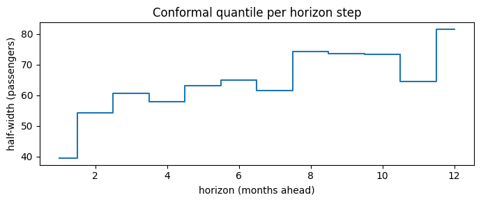
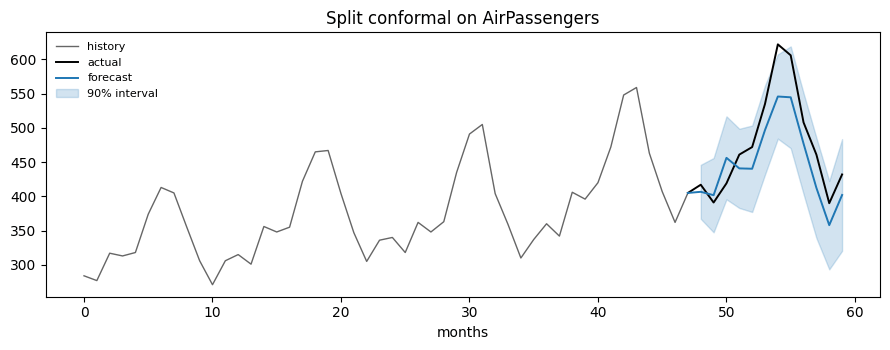
calibrate_cv returned a new fitted object and left method untouched; its score_quantile_ is that q, one per (series, horizon) cell. Plotting it against the horizon shows the band widening as the ETS forecast has more room to drift.

q = fitted.score_quantile_[0]

fig, ax = plt.subplots(figsize=(7, 3))
ax.step(np.arange(1, HORIZON + 1), q, where="mid", color="C0")
ax.set_xlabel("horizon (months ahead)")
ax.set_ylabel("half-width (passengers)")
ax.set_title("Conformal quantile per horizon step")
fig.tight_layout()

prediction = fitted.predict(panel[:, :cutoff])

tail = panel[0, cutoff - 48 : cutoff]
past = np.arange(len(tail))
future = np.arange(len(tail), len(tail) + HORIZON)
join = np.r_[past[-1], future]

fig, ax = plt.subplots(figsize=(9, 3.6))
ax.plot(past, tail, color="0.4", lw=1, label="history")
ax.plot(join, np.r_[tail[-1], panel[0, cutoff:]], color="k", lw=1.4, label="actual")
ax.plot(join, np.r_[tail[-1], prediction.point[0, 0]], color="C0", lw=1.4, label="forecast")
ax.fill_between(
    future,
    prediction.interval[0, 0, :, 0],
    prediction.interval[0, 0, :, 1],
    color="C0",
    alpha=0.2,
    label="90% interval",
)
ax.set_title("Split conformal on AirPassengers")
ax.set_xlabel("months")
ax.legend(loc="upper left", fontsize=8, frameon=False)
fig.tight_layout()

Measured coverage

N_HOLDOUT = 4
histories, truths = [], []
for k in range(N_HOLDOUT):
    end = panel.shape[1] - (N_HOLDOUT - k) * HORIZON
    histories.append(panel[:, :end])
    truths.append(panel[:, end : end + HORIZON])

report = evaluate(fitted, histories, np.stack(truths, axis=1))
print(report.summary())

Report — SplitConformal
  target coverage: 0.900
  marginal coverage: 0.938
  coverage by horizon: [1.000, 1.000, 1.000, 1.000, 1.000, 1.000, 0.500, 0.750, 1.000, 1.000, 1.000, 1.000]
  mean width: 128.190
  mean Winkler score: 149.198
  n_holdout_samples: 4

Asymmetric intervals

Everything above builds an equal-width band centred on the forecast, because the absolute residual |y - ŷ| throws away the sign of the error. It targets total coverage 1 - alpha and says nothing about how the misses split between the tails: with skewed residuals one tail can take nearly all of them. And the symmetric band has a cost: a forecaster that is biased — consistently high or consistently low — can only be covered by widening the band on both sides, including the side the errors never fall on. symmetric=False scores the signed residual r = y - ŷ instead and takes one one-sided conformal quantile per tail:

lower_offset = the alpha_lo quantile of r_1 ... r_n
upper_offset = the alpha_hi quantile of the same r

with the same n + 1 correction as before, and the interval becomes [ŷ + lower_offset, ŷ + upper_offset]. Both offsets are stored per (series, horizon) cell, so score_quantile_ gains a trailing axis of size 2. Nothing constrains them to be mirror images, so the band can shift as well as widen. The two levels are bound by alpha_lo + (1 - alpha_hi) == alpha: the tails move against each other on a fixed budget, and both are mandatory once symmetric=False. Setting them to alpha/2 each — 0.05 and 0.95 here — gives the equal-tailed interval: the same total alpha as the symmetric fit, but now alpha/2 per tail, and the band is no longer forced to be centred. The price is calibration data — each tail needs at least ceil(2 / alpha) windows per series instead of ceil(1 / alpha).

asym = SplitConformal(alpha=ALPHA, symmetric=False, alpha_lo=0.05, alpha_hi=0.95)
asym_fitted = asym.calibrate_cv(forecaster, n_windows=24)

q_asym = asym_fitted.score_quantile_[0]
print("score_quantile_ shape:", q_asym.shape, "-> (horizon, [lower, upper])\n")

signed = fitted.truths_calibration_ - fitted.predictions_calibration_
print(f"share of calibration residuals above the forecast: {np.mean(signed > 0):.1%}")
print(f"mean signed residual: {np.mean(signed):+.1f} passengers\n")

print(f"{'h':>3}  {'lower':>8} {'upper':>8}  {'width':>7}  {'symmetric':>9}")
for h in (0, 5, 11):
    lo, hi = q_asym[h]
    print(f"{h + 1:>3}  {lo:>8.1f} {hi:>8.1f}  {hi - lo:>7.1f}  {2 * q[h]:>9.1f}")
width_asym, width_sym = q_asym[:, 1] - q_asym[:, 0], 2 * q
print(f"\nmean width  asymmetric {width_asym.mean():.1f}  vs symmetric {width_sym.mean():.1f}")
print(f"narrower at {(width_asym < width_sym).sum()} of {HORIZON} steps")
print(f"highest lower offset: {q_asym[:, 0].max():+.1f} at step {q_asym[:, 0].argmax() + 1}")

score_quantile_ shape: (12, 2) -> (horizon, [lower, upper])

share of calibration residuals above the forecast: 74.3%
mean signed residual: +19.5 passengers

  h     lower    upper    width  symmetric
  1     -22.1     45.1     67.2       78.8
  6     -33.4     68.2    101.6      130.0
 12      -4.4     82.2     86.6      163.2

mean width  asymmetric 102.2  vs symmetric 128.2
narrower at 11 of 12 steps
highest lower offset: -2.5 at step 11

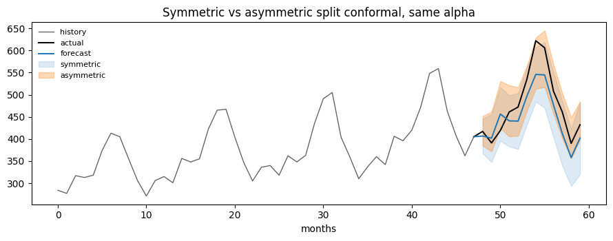
AutoETS under-forecasts AirPassengers, so most calibration residuals land above the forecast. The symmetric band has to reach that far above and the same distance below, where almost nothing falls. The asymmetric band puts its mass where the errors are, and is narrower at eleven of the twelve steps at the same total alpha — the fourth step is a dead heat, and none of them is meaningfully wider. The gap is widest at the long end, where the bias has had the most room to accumulate: at the twelfth step the asymmetric band is barely half the width.

pred_asym = asym_fitted.predict(panel[:, :cutoff])

fig, ax = plt.subplots(figsize=(9, 3.6))
ax.plot(past, tail, color="0.4", lw=1, label="history")
ax.plot(join, np.r_[tail[-1], panel[0, cutoff:]], color="k", lw=1.4, label="actual")
ax.plot(join, np.r_[tail[-1], prediction.point[0, 0]], color="C0", lw=1.4, label="forecast")
ax.fill_between(
    future,
    prediction.interval[0, 0, :, 0],
    prediction.interval[0, 0, :, 1],
    color="C0",
    alpha=0.15,
    label="symmetric",
)
ax.fill_between(
    future,
    pred_asym.interval[0, 0, :, 0],
    pred_asym.interval[0, 0, :, 1],
    color="C1",
    alpha=0.30,
    label="asymmetric",
)
ax.set_title("Symmetric vs asymmetric split conformal, same alpha")
ax.set_xlabel("months")
ax.legend(loc="upper left", fontsize=8, frameon=False)
fig.tight_layout()

On the same holdout measured earlier:

asym_report = evaluate(asym_fitted, histories, np.stack(truths, axis=1))
print(asym_report.summary())

Report — SplitConformal
  target coverage: 0.900
  marginal coverage: 0.979
  coverage by horizon: [1.000, 1.000, 0.750, 1.000, 1.000, 1.000, 1.000, 1.000, 1.000, 1.000, 1.000, 1.000]
  mean width: 102.243
  mean Winkler score: 104.610
  n_holdout_samples: 4

Narrower on average and better covered, with a lower Winkler score — which is the combination that says the symmetric band was paying for width it did not need. Do not read too much into four holdout windows; the point is the direction, and the mechanism behind it is visible in the offsets above.

The calibration data has to stretch further

Each tail is now its own one-sided quantile, so each enforces its own ceil(1 / level) floor. The binding requirement is the stricter of the two:

max(ceil(1 / alpha_lo), ceil(1 / (1 - alpha_hi)))

For the even split that is ceil(1 / 0.05) = 20, comfortably under the 24 windows this page calibrates on. Tilt the budget toward the lower tail and the floor moves fast:

from conformalforecast.base import InsufficientCalibrationSamples

try:
    tilted = SplitConformal(alpha=ALPHA, symmetric=False, alpha_lo=0.02, alpha_hi=0.92)
    tilted.calibrate_cv(forecaster, n_windows=24)
except InsufficientCalibrationSamples as err:
    print(f"{type(err).__name__}: {err}")
    print("series:", err.series_indices)

InsufficientCalibrationSamples: Series [0] have fewer than ceil(1/alpha) = 50 effective calibration samples for alpha=0.02 (from alpha_lo=0.02).
series: [0]

alpha_lo=0.02 needs 50 calibration windows on its own, and the message names alpha_lo rather than quoting the alpha you passed — the failing knob is the one you want to see. Budget for it: an asymmetric interval with a narrow tail needs several times the calibration data a symmetric one at the same alpha would.

A one-sided interval means the forecaster is biased If both offsets come out with the same sign, the interval lies entirely above or entirely below the point forecast, and fit warns:
Asymmetric split conformal produced an interval lying entirely on one side of
the point forecast. The forecaster is biased on this calibration data; the
interval is shifting rather than widening to compensate.
That is not a defect in the method — it is the method reporting one in the forecaster, and the offsets it produces are still valid. The fit above does not trip it, but not by much: its highest lower offset is -2.5, at the eleventh step, so a little more drift would put the whole band above the forecast. Fix the bias in the model if you can; conformalizing around it works, but it spends interval width on a problem a better point forecast would not have.

Use symmetric=False when one tail carries the real cost — inventory, staffing, capacity — or when the forecaster is biased and you would rather shift than widen. Stay symmetric otherwise: it needs less calibration data, and an uninformative tilt just moves coverage around. When the asymmetry depends on the features of each step rather than being a constant offset, that is CQR’s job, not this one.

Using the array surface

The forecaster surface did three things above: ran the cross-validation, converted Nixtla frames to arrays, and called the calibration math. If your library already owns the first two — which is the case inside statsforecast, mlforecast and neuralforecast — you want the array surface: fit(predictions, truths) on the method returns the same kind of fitted object, and interval(predictions) on that object applies it — no forecaster and no adapter anywhere in the signature.

# Reuse the calibration arrays the forecaster surface already assembled.
predictions = fitted.predictions_calibration_
observed = fitted.truths_calibration_
print("calibration arrays:", predictions.shape, "(n_series, n_windows, horizon)")

array_fitted = SplitConformal(alpha=ALPHA).fit(predictions, observed)
interval = array_fitted.interval(prediction.point)

print("interval", interval.shape)
np.testing.assert_allclose(interval, prediction.interval)
print("identical to the forecaster-surface result")

calibration arrays: (1, 24, 12) (n_series, n_windows, horizon)
interval (1, 1, 12, 2)
identical to the forecaster-surface result

When not to use it

Your coverage drifts over time. Split conformal calibrates once and never looks again, so a regime change leaves it silently mis-calibrated. Use ACI, AgACI or NexCP.
Your errors are strongly heteroscedastic. The absolute-residual score makes one constant-width band per cell. If the noise scales with the level, that band is wrong nearly everywhere. Use CQR.
You need the width itself to be informative. A constant band cannot say “this particular step is unusually uncertain”. Use SPCI.

None of these are reasons to skip split conformal first — it is the measurement that tells you which of the three problems you actually have.

References

H. Papadopoulos, Kostas Proedrou, V. Vovk, and A. Gammerman, “Inductive Confidence Machines for Regression,” pp. 345–356, Jan. 2002, doi: 10.1007/3-540-36755-1_29.
V. Vovk, A. Gammerman, and G. Shafer, Algorithmic Learning in a Random World. Springer Nature, 2005. doi: 10.1007/b106715.
J. Lei, M. G’Sell, A. Rinaldo, R. J. Tibshirani, and L. Wasserman, “Distribution-Free Predictive Inference For Regression,” 2016. https://arxiv.org/abs/1604.04173

CQR — the other offline method, for heteroscedastic errors.
Methods overview — the decision guide.
Diagnostics — measuring an interval properly.

Getting Started

Concepts

Capabilities

Methods

Nixtlaverse

API Reference

Split conformal

What it does

Worked example

Measured coverage

Asymmetric intervals

The calibration data has to stretch further

Using the array surface

When not to use it

References

Next

​What it does

​Worked example

​Measured coverage

​Asymmetric intervals

​The calibration data has to stretch further

​Using the array surface

​When not to use it

​References

​Next

What it does

Worked example

Measured coverage

Asymmetric intervals

The calibration data has to stretch further

Using the array surface

When not to use it

References

Next