exogenous parameter, so you can build test panels that exercise a
model’s covariate handling end to end, all reproducible from the seed.
Three kinds of covariate
- Datetime features — calendar and cyclical (sin/cos) time encodings, added frequency-aware.
- Pattern-injection flags — binary
anomaly_flag/changepoint_flag/missing_flagcolumns marking exactly where each injected pattern landed (ground-truth labels for detectors).- Correlated exogenous — numeric columns statistically tied to the target series.
import matplotlib.pyplot as plt
import numpy as np
import polars as pl

from synforecast.exogenous import CorrelatedExogConfig, ExogenousConfig
from synforecast.generators import RandomWalkGenerator
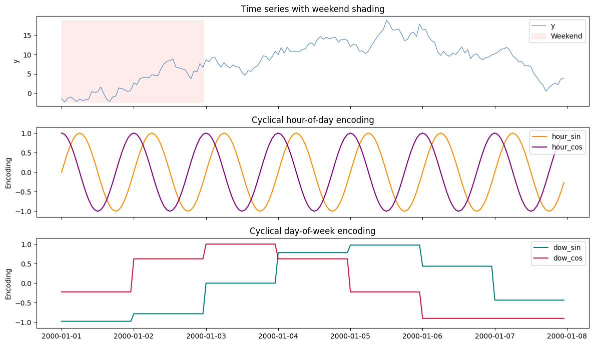
Datetime features
Enabledatetime_features for calendar columns (year, month,
day_of_week, hour, etc.) and datetime_cyclical for sin/cos encodings.
Features are frequency-aware: hourly data includes hour,
hour_sin/cos; daily data omits them since they would be constant.
gen = RandomWalkGenerator(engine="polars", **{
    "min_length": 168,  # 7 days of hourly data
    "max_length": 168,
    "freq": "h",
    "seed": 42,
    "exogenous": ExogenousConfig(
        datetime_features=True,
        datetime_cyclical=True,
    ),
})
df = gen.generate(n_series=1)

print(f"Columns: {df.columns}")
df.head(10)
Columns: ['unique_id', 'ds', 'y', 'year', 'quarter', 'month', 'day_of_year', 'day_of_week', 'day_of_month', 'is_weekend', 'hour', 'hour_sin', 'hour_cos', 'dow_sin', 'dow_cos', 'month_sin', 'month_cos', 'doy_sin', 'doy_cos']
| unique_id | ds | y | year | quarter | month | day_of_year | day_of_week | day_of_month | is_weekend | hour | hour_sin | hour_cos | dow_sin | dow_cos | month_sin | month_cos | doy_sin | doy_cos |
|---|---|---|---|---|---|---|---|---|---|---|---|---|---|---|---|---|---|---|
| cat | datetime[ns] | f64 | i32 | i8 | i8 | i16 | i8 | i8 | i8 | i8 | f32 | f32 | f32 | f32 | f32 | f32 | f32 | f32 |
| ”0” | 2000-01-01 00:00:00 | -1.401594 | 2000 | 1 | 1 | 1 | 5 | 1 | 1 | 0 | 0.0 | 1.0 | -0.974928 | -0.222521 | 0.0 | 1.0 | 0.0 | 1.0 |
| ”0” | 2000-01-01 01:00:00 | -2.307539 | 2000 | 1 | 1 | 1 | 5 | 1 | 1 | 1 | 0.258819 | 0.965926 | -0.974928 | -0.222521 | 0.0 | 1.0 | 0.0 | 1.0 |
| ”0” | 2000-01-01 02:00:00 | -1.352484 | 2000 | 1 | 1 | 1 | 5 | 1 | 1 | 2 | 0.5 | 0.866025 | -0.974928 | -0.222521 | 0.0 | 1.0 | 0.0 | 1.0 |
| ”0” | 2000-01-01 03:00:00 | -1.011828 | 2000 | 1 | 1 | 1 | 5 | 1 | 1 | 3 | 0.707107 | 0.707107 | -0.974928 | -0.222521 | 0.0 | 1.0 | 0.0 | 1.0 |
| ”0” | 2000-01-01 04:00:00 | -1.511372 | 2000 | 1 | 1 | 1 | 5 | 1 | 1 | 4 | 0.866025 | 0.5 | -0.974928 | -0.222521 | 0.0 | 1.0 | 0.0 | 1.0 |
| ”0” | 2000-01-01 05:00:00 | -2.176202 | 2000 | 1 | 1 | 1 | 5 | 1 | 1 | 5 | 0.965926 | 0.258819 | -0.974928 | -0.222521 | 0.0 | 1.0 | 0.0 | 1.0 |
| ”0” | 2000-01-01 06:00:00 | -1.574639 | 2000 | 1 | 1 | 1 | 5 | 1 | 1 | 6 | 1.0 | 6.1232e-17 | -0.974928 | -0.222521 | 0.0 | 1.0 | 0.0 | 1.0 |
| ”0” | 2000-01-01 07:00:00 | -1.915517 | 2000 | 1 | 1 | 1 | 5 | 1 | 1 | 7 | 0.965926 | -0.258819 | -0.974928 | -0.222521 | 0.0 | 1.0 | 0.0 | 1.0 |
| ”0” | 2000-01-01 08:00:00 | -1.746987 | 2000 | 1 | 1 | 1 | 5 | 1 | 1 | 8 | 0.866025 | -0.5 | -0.974928 | -0.222521 | 0.0 | 1.0 | 0.0 | 1.0 |
| ”0” | 2000-01-01 09:00:00 | -1.566314 | 2000 | 1 | 1 | 1 | 5 | 1 | 1 | 9 | 0.707107 | -0.707107 | -0.974928 | -0.222521 | 0.0 | 1.0 | 0.0 | 1.0 |
ts = df["ds"].to_list()
y = df["y"].to_numpy()
is_weekend = df["is_weekend"].to_numpy().astype(bool)

fig, axes = plt.subplots(3, 1, figsize=(12, 7), sharex=True)

# Panel 1: time series with weekend shading
axes[0].plot(ts, y, linewidth=0.8, color="steelblue", label="y")
axes[0].fill_between(ts, y.min(), y.max(), where=is_weekend,
                      alpha=0.15, color="salmon", label="Weekend")
axes[0].set_ylabel("y")
axes[0].set_title("Time series with weekend shading")
axes[0].legend(loc="upper right")

# Panel 2: hour-of-day cyclical encoding
axes[1].plot(ts, df["hour_sin"].to_numpy(), label="hour_sin", color="darkorange")
axes[1].plot(ts, df["hour_cos"].to_numpy(), label="hour_cos", color="purple")
axes[1].set_ylabel("Encoding")
axes[1].set_title("Cyclical hour-of-day encoding")
axes[1].legend(loc="upper right")
axes[1].set_ylim(-1.15, 1.15)

# Panel 3: day-of-week cyclical encoding
axes[2].plot(ts, df["dow_sin"].to_numpy(), label="dow_sin", color="teal")
axes[2].plot(ts, df["dow_cos"].to_numpy(), label="dow_cos", color="crimson")
axes[2].set_ylabel("Encoding")
axes[2].set_title("Cyclical day-of-week encoding")
axes[2].legend(loc="upper right")
axes[2].set_ylim(-1.15, 1.15)

plt.tight_layout()
plt.show()
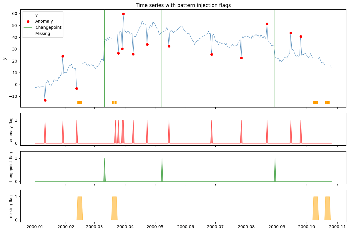
Pattern injection flags
When pattern injection is enabled (anomalies, changepoints, missing data), you can get binary flag columns indicating exactly where each pattern was injected. This is useful for training anomaly detectors or evaluating changepoint detection algorithms.gen = RandomWalkGenerator(engine="polars", **{
"min_length": 300,
"max_length": 300,
"freq": "D",
"seed": 42,
"drift": 0.1,
"volatility": 1.5,
"anomalies": True,
"anomaly_fraction": 0.05,
"anomaly_types": ["spike", "dip"],
"spike_magnitude": 15.0,
"dip_magnitude": -15.0,
"changepoints": True,
"num_changepoints": 3,
"changepoint_type": "level",
"missing_data": True,
"missing_rate": 0.08,
"missing_pattern": "block",
"missing_block_size": 5,
"exogenous": ExogenousConfig(
anomaly_flags=True,
changepoint_flags=True,
missing_flags=True,
),
})
df = gen.generate(n_series=1)
print(f"Columns: {df.columns}")
print(f"Anomalies: {df['anomaly_flag'].sum()}, "
f"Changepoints: {df['changepoint_flag'].sum()}, "
f"Missing: {df['missing_flag'].sum()}")
df.head(10)
Columns: ['unique_id', 'ds', 'y', 'anomaly_flag', 'changepoint_flag', 'missing_flag']
Anomalies: 15, Changepoints: 3, Missing: 20
| unique_id | ds | y | anomaly_flag | changepoint_flag | missing_flag |
|---|---|---|---|---|---|
| cat | datetime[ns] | f64 | i8 | i8 | i8 |
| ”0” | 2000-01-01 00:00:00 | -2.002391 | 0 | 0 | 0 |
| ”0” | 2000-01-02 00:00:00 | -3.261309 | 0 | 0 | 0 |
| ”0” | 2000-01-03 00:00:00 | -1.728725 | 0 | 0 | 0 |
| ”0” | 2000-01-04 00:00:00 | -1.117742 | 0 | 0 | 0 |
| ”0” | 2000-01-05 00:00:00 | -1.767059 | 0 | 0 | 0 |
| ”0” | 2000-01-06 00:00:00 | -2.664304 | 0 | 0 | 0 |
| ”0” | 2000-01-07 00:00:00 | -1.661958 | 0 | 0 | 0 |
| ”0” | 2000-01-08 00:00:00 | -2.073275 | 0 | 0 | 0 |
| ”0” | 2000-01-09 00:00:00 | -1.72048 | 0 | 0 | 0 |
| ”0” | 2000-01-10 00:00:00 | -1.34947 | 0 | 0 | 0 |
ts = df["ds"].to_list()
y = df["y"].to_numpy()
anom = df["anomaly_flag"].to_numpy().astype(bool)
cp = df["changepoint_flag"].to_numpy().astype(bool)
miss = df["missing_flag"].to_numpy().astype(bool)

fig, axes = plt.subplots(4, 1, figsize=(12, 8), sharex=True,
                          gridspec_kw={"height_ratios": [3, 1, 1, 1]})

# Panel 1: time series with flagged points
axes[0].plot(ts, y, linewidth=0.7, color="steelblue", label="y", zorder=1)
if anom.any():
    axes[0].scatter([ts[i] for i in range(len(ts)) if anom[i]],
                    y[anom], color="red", s=30, zorder=3, label="Anomaly")
if cp.any():
    for i, t_cp in enumerate([ts[i] for i in range(len(ts)) if cp[i]]):
        axes[0].axvline(t_cp, color="green", linewidth=1.2, alpha=0.7,
                        label="Changepoint" if i == 0 else None)
if miss.any():
    axes[0].scatter([ts[i] for i in range(len(ts)) if miss[i]],
                    np.full(miss.sum(), np.nanmin(y) - 2),
                    marker="|", color="orange", s=40, zorder=2, label="Missing")
axes[0].set_ylabel("y")
axes[0].set_title("Time series with pattern injection flags")
axes[0].legend(loc="upper left")

# Panels 2-4: binary flag traces
for ax, (name, flag, color) in zip(
    axes[1:],
    [("anomaly_flag", anom, "red"),
     ("changepoint_flag", cp, "green"),
     ("missing_flag", miss, "orange")],
):
    ax.fill_between(ts, 0, flag.astype(int), color=color, alpha=0.5)
    ax.set_ylabel(name, fontsize=9)
    ax.set_ylim(-0.1, 1.3)
    ax.set_yticks([0, 1])

plt.tight_layout()
plt.show()
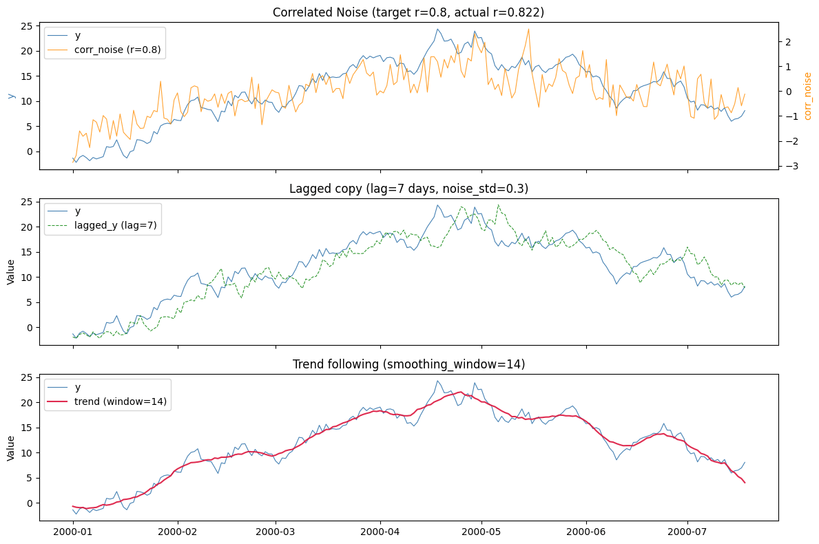
Correlated exogenous variables
Generate additional numeric columns that are statistically related to the target series. Three methods are available:| Method | Description |
|---|---|
correlated_noise | Cholesky-based noise with a target Pearson correlation |
lagged_copy | Shifted copy of the target series with additive noise |
trend_following | Moving-average smoothing of the target |
These are derived from the target Each correlated column is computed fromy— a correlated draw, a lagged copy, or a smoothed trend — so it carries information about the target by construction. That is exactly what you want when testing whether a model can exploit covariates. But treat them accordingly: alagged_copywithlag=7is only a leak-free feature for a real forecast if the lag exceeds the forecast horizon.
gen = RandomWalkGenerator(engine="polars", **{
    "min_length": 200,
    "max_length": 200,
    "freq": "D",
    "seed": 42,
    "drift": 0.05,
    "volatility": 1.0,
    "exogenous": ExogenousConfig(
        correlated=[
            CorrelatedExogConfig(
                name="corr_noise",
                method="correlated_noise",
                correlation=0.8,
            ),
            CorrelatedExogConfig(
                name="lagged_y",
                method="lagged_copy",
                lag=7,
                noise_std=0.3,
            ),
            CorrelatedExogConfig(
                name="trend",
                method="trend_following",
                smoothing_window=14,
                trend_noise_std=0.1,
            ),
        ]
    ),
})
df = gen.generate(n_series=1)

print(f"Columns: {df.columns}")
y = df["y"].to_numpy()
corr = np.corrcoef(y, df["corr_noise"].to_numpy())[0, 1]
print(f"Target correlation: 0.8, actual: {corr:.3f}")
df.head(10)
Columns: ['unique_id', 'ds', 'y', 'corr_noise', 'lagged_y', 'trend']
Target correlation: 0.8, actual: 0.822
| unique_id | ds | y | corr_noise | lagged_y | trend |
|---|---|---|---|---|---|
| cat | datetime[ns] | f64 | f64 | f64 | f64 |
| ”0” | 2000-01-01 00:00:00 | -1.351594 | -2.863126 | -1.966645 | -0.657573 |
| ”0” | 2000-01-02 00:00:00 | -2.207539 | -2.581491 | -2.222155 | -0.844525 |
| ”0” | 2000-01-03 00:00:00 | -1.202484 | -1.597043 | -1.455453 | -0.922337 |
| ”0” | 2000-01-04 00:00:00 | -0.811828 | -1.814348 | -1.177472 | -0.903796 |
| ”0” | 2000-01-05 00:00:00 | -1.261372 | -1.691236 | -1.524818 | -1.119365 |
| ”0” | 2000-01-06 00:00:00 | -1.876202 | -2.270328 | -1.976439 | -0.993435 |
| ”0” | 2000-01-07 00:00:00 | -1.224639 | -1.148895 | -0.949868 | -0.943064 |
| ”0” | 2000-01-08 00:00:00 | -1.515517 | -1.246452 | -1.749512 | -0.86473 |
| ”0” | 2000-01-09 00:00:00 | -1.296987 | -1.646017 | -2.19835 | -0.558921 |
| ”0” | 2000-01-10 00:00:00 | -1.066314 | -0.980272 | -1.347734 | -0.315824 |
ts = df["ds"].to_list()
y = df["y"].to_numpy()

fig, axes = plt.subplots(3, 1, figsize=(12, 8), sharex=True)

# Panel 1: correlated noise
ax = axes[0]
ax.plot(ts, y, linewidth=0.8, color="steelblue", label="y")
ax2 = ax.twinx()
ax2.plot(ts, df["corr_noise"].to_numpy(), linewidth=0.8,
         color="darkorange", alpha=0.8, label="corr_noise (r=0.8)")
ax.set_ylabel("y", color="steelblue")
ax2.set_ylabel("corr_noise", color="darkorange")
corr = np.corrcoef(y, df["corr_noise"].to_numpy())[0, 1]
ax.set_title(f"Correlated Noise (target r=0.8, actual r={corr:.3f})")
lines1, labels1 = ax.get_legend_handles_labels()
lines2, labels2 = ax2.get_legend_handles_labels()
ax.legend(lines1 + lines2, labels1 + labels2, loc="upper left")

# Panel 2: lagged copy
ax = axes[1]
ax.plot(ts, y, linewidth=0.8, color="steelblue", label="y")
ax.plot(ts, df["lagged_y"].to_numpy(), linewidth=0.8,
        color="green", alpha=0.8, linestyle="--", label="lagged_y (lag=7)")
ax.set_ylabel("Value")
ax.set_title("Lagged copy (lag=7 days, noise_std=0.3)")
ax.legend(loc="upper left")

# Panel 3: trend following
ax = axes[2]
ax.plot(ts, y, linewidth=0.8, color="steelblue", label="y")
ax.plot(ts, df["trend"].to_numpy(), linewidth=1.5,
        color="crimson", alpha=0.9, label="trend (window=14)")
ax.set_ylabel("Value")
ax.set_title("Trend following (smoothing_window=14)")
ax.legend(loc="upper left")

plt.tight_layout()
plt.show()
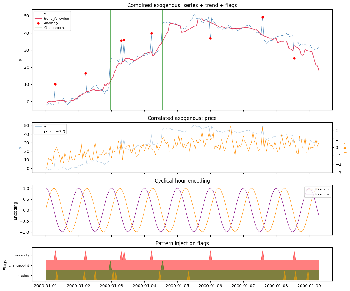
Combined: all exogenous types
All exogenous types can be combined freely in a single generator call.gen = RandomWalkGenerator(engine="polars", **{
"min_length": 200,
"max_length": 200,
"freq": "h",
"seed": 42,
"drift": 0.02,
"volatility": 1.0,
"anomalies": True,
"anomaly_fraction": 0.04,
"spike_magnitude": 12.0,
"dip_magnitude": -12.0,
"changepoints": True,
"num_changepoints": 2,
"missing_data": True,
"missing_rate": 0.05,
"exogenous": ExogenousConfig(
datetime_features=True,
datetime_cyclical=True,
anomaly_flags=True,
changepoint_flags=True,
missing_flags=True,
correlated=[
CorrelatedExogConfig(name="price", correlation=0.7),
CorrelatedExogConfig(
name="trend",
method="trend_following",
smoothing_window=12,
trend_noise_std=0.05,
),
],
),
})
df = gen.generate(n_series=1)
print(f"Generated DataFrame: {df.shape[0]} rows x {df.shape[1]} columns")
print(f"Columns: {df.columns}")
df.head(10)
Generated DataFrame: 200 rows x 24 columns
Columns: ['unique_id', 'ds', 'y', 'anomaly_flag', 'changepoint_flag', 'missing_flag', 'year', 'quarter', 'month', 'day_of_year', 'day_of_week', 'day_of_month', 'is_weekend', 'hour', 'hour_sin', 'hour_cos', 'dow_sin', 'dow_cos', 'month_sin', 'month_cos', 'doy_sin', 'doy_cos', 'price', 'trend']
| unique_id | ds | y | anomaly_flag | changepoint_flag | missing_flag | year | quarter | month | day_of_year | day_of_week | day_of_month | is_weekend | hour | hour_sin | hour_cos | dow_sin | dow_cos | month_sin | month_cos | doy_sin | doy_cos | price | trend |
|---|---|---|---|---|---|---|---|---|---|---|---|---|---|---|---|---|---|---|---|---|---|---|---|
| cat | datetime[ns] | f64 | i8 | i8 | i8 | i32 | i8 | i8 | i16 | i8 | i8 | i8 | i8 | f32 | f32 | f32 | f32 | f32 | f32 | f32 | f32 | f64 | f64 |
| ”0” | 2000-01-01 00:00:00 | -1.381594 | 0 | 0 | 0 | 2000 | 1 | 1 | 1 | 5 | 1 | 1 | 0 | 0.0 | 1.0 | -0.974928 | -0.222521 | 0.0 | 1.0 | 0.0 | 1.0 | -2.731882 | -0.880927 |
| ”0” | 2000-01-01 01:00:00 | -2.267539 | 0 | 0 | 0 | 2000 | 1 | 1 | 1 | 5 | 1 | 1 | 1 | 0.258819 | 0.965926 | -0.974928 | -0.222521 | 0.0 | 1.0 | 0.0 | 1.0 | -2.306626 | -0.900407 |
| ”0” | 2000-01-01 02:00:00 | -1.292484 | 0 | 0 | 0 | 2000 | 1 | 1 | 1 | 5 | 1 | 1 | 2 | 0.5 | 0.866025 | -0.974928 | -0.222521 | 0.0 | 1.0 | 0.0 | 1.0 | -1.243434 | -0.086426 |
| ”0” | 2000-01-01 03:00:00 | -0.931828 | 0 | 0 | 0 | 2000 | 1 | 1 | 1 | 5 | 1 | 1 | 3 | 0.707107 | 0.707107 | -0.974928 | -0.222521 | 0.0 | 1.0 | 0.0 | 1.0 | -1.545055 | -0.105205 |
| ”0” | 2000-01-01 04:00:00 | -1.411372 | 0 | 0 | 0 | 2000 | 1 | 1 | 1 | 5 | 1 | 1 | 4 | 0.866025 | 0.5 | -0.974928 | -0.222521 | 0.0 | 1.0 | 0.0 | 1.0 | -1.351844 | -0.202032 |
| ”0” | 2000-01-01 05:00:00 | -2.056202 | 0 | 0 | 0 | 2000 | 1 | 1 | 1 | 5 | 1 | 1 | 5 | 0.965926 | 0.258819 | -0.974928 | -0.222521 | 0.0 | 1.0 | 0.0 | 1.0 | -1.976786 | -0.124526 |
| ”0” | 2000-01-01 06:00:00 | -1.434639 | 0 | 0 | 0 | 2000 | 1 | 1 | 1 | 5 | 1 | 1 | 6 | 1.0 | 6.1232e-17 | -0.974928 | -0.222521 | 0.0 | 1.0 | 0.0 | 1.0 | -0.712831 | -0.026375 |
| ”0” | 2000-01-01 07:00:00 | 10.244483 | 1 | 0 | 0 | 2000 | 1 | 1 | 1 | 5 | 1 | 1 | 7 | 0.965926 | -0.258819 | -0.974928 | -0.222521 | 0.0 | 1.0 | 0.0 | 1.0 | -0.282877 | 0.024575 |
| ”0” | 2000-01-01 08:00:00 | NaN | 0 | 0 | 1 | 2000 | 1 | 1 | 1 | 5 | 1 | 1 | 8 | 0.866025 | -0.5 | -0.974928 | -0.222521 | 0.0 | 1.0 | 0.0 | 1.0 | 0.047155 | 0.437111 |
| ”0” | 2000-01-01 09:00:00 | -1.366314 | 0 | 0 | 0 | 2000 | 1 | 1 | 1 | 5 | 1 | 1 | 9 | 0.707107 | -0.707107 | -0.974928 | -0.222521 | 0.0 | 1.0 | 0.0 | 1.0 | -0.532896 | 0.532599 |
ts = df["ds"].to_list()
y = df["y"].to_numpy()
anom = df["anomaly_flag"].to_numpy().astype(bool)
cp = df["changepoint_flag"].to_numpy().astype(bool)
miss = df["missing_flag"].to_numpy().astype(bool)

fig, axes = plt.subplots(4, 1, figsize=(12, 10), sharex=True,
                          gridspec_kw={"height_ratios": [3, 1.5, 1.5, 1]})

# Panel 1: main series + trend + anomaly/changepoint markers
ax = axes[0]
ax.plot(ts, y, linewidth=0.7, color="steelblue", label="y")
ax.plot(ts, df["trend"].to_numpy(), linewidth=1.5, color="crimson",
        alpha=0.8, label="trend_following")
if anom.any():
    ax.scatter([ts[i] for i in range(len(ts)) if anom[i]],
              y[anom], color="red", s=25, zorder=3, label="Anomaly")
if cp.any():
    for i, t_cp in enumerate([ts[i] for i in range(len(ts)) if cp[i]]):
        ax.axvline(t_cp, color="green", linewidth=1, alpha=0.6,
                   label="Changepoint" if i == 0 else None)
ax.set_ylabel("y")
ax.set_title("Combined exogenous: series + trend + flags")
ax.legend(loc="upper left", fontsize=8)

# Panel 2: correlated price
ax = axes[1]
ax.plot(ts, y, linewidth=0.6, color="steelblue", alpha=0.5, label="y")
ax2 = ax.twinx()
ax2.plot(ts, df["price"].to_numpy(), linewidth=0.7,
         color="darkorange", label="price (r=0.7)")
ax.set_ylabel("y", color="steelblue")
ax2.set_ylabel("price", color="darkorange")
lines1, labels1 = ax.get_legend_handles_labels()
lines2, labels2 = ax2.get_legend_handles_labels()
ax.legend(lines1 + lines2, labels1 + labels2, loc="upper left", fontsize=8)
ax.set_title("Correlated exogenous: price")

# Panel 3: cyclical hour encoding
ax = axes[2]
ax.plot(ts, df["hour_sin"].to_numpy(), linewidth=0.8,
        color="darkorange", label="hour_sin")
ax.plot(ts, df["hour_cos"].to_numpy(), linewidth=0.8,
        color="purple", label="hour_cos")
ax.set_ylabel("Encoding")
ax.set_ylim(-1.15, 1.15)
ax.set_title("Cyclical hour encoding")
ax.legend(loc="upper right", fontsize=8)

# Panel 4: combined binary flags
ax = axes[3]
ax.fill_between(ts, 0, anom.astype(int) * 0.9 + 2.0,
                color="red", alpha=0.5, label="anomaly")
ax.fill_between(ts, 0, cp.astype(int) * 0.9 + 1.0,
                color="green", alpha=0.5, label="changepoint")
ax.fill_between(ts, 0, miss.astype(int) * 0.9,
                color="orange", alpha=0.5, label="missing")
ax.set_ylabel("Flags")
ax.set_yticks([0.45, 1.45, 2.45])
ax.set_yticklabels(["missing", "changepoint", "anomaly"], fontsize=8)
ax.set_ylim(-0.1, 3.2)
ax.set_title("Pattern injection flags")

plt.tight_layout()
plt.show()