

StateSpaceGenerator lets you specify
the transition and observation dynamics directly to build custom linear
systems.
The model xt=Fxt−1+wt,wt∼(0,Q),yt=Hxt+vt,vt∼N(0,R) A latent state evolves by a linear transition with process noise, and is mapped to the observed series by an observation equation with measurement noise. Choosing these dynamics reproduces local-level, local-trend, and other structural time-series models.
import numpy as np
import polars as pl
import matplotlib.pyplot as plt

from synforecast.generators import StateSpaceGenerator
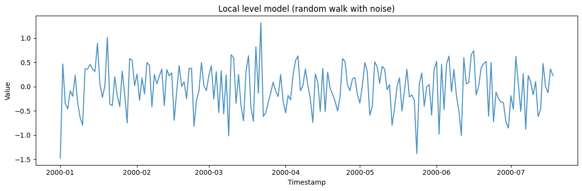
1. Basic local level model (random walk with noise)
The simplest state space model: a hidden random walk observed with measurement noise.local_level_params = {
"min_length": 200,
"max_length": 200,
"freq": "D",
"state_dim": 1,
"obs_dim": 1,
"seed": 42,
}
local_level_gen = StateSpaceGenerator(engine="polars", **local_level_params)
local_level_df = local_level_gen.generate(n_series=1)
print(f"Generated {len(local_level_df)} observations from local level model")
print(
f"Statistics: Mean={local_level_df['y'].mean():.4f}, "
f"Std={local_level_df['y'].std():.4f}"
)
local_level_df.head(10)
Generated 200 observations from local level model
Statistics: Mean=-0.0235, Std=0.4556
| unique_id | ds | y |
|---|---|---|
| cat | datetime[ns] | f64 |
| ”0” | 2000-01-01 00:00:00 | -1.477252 |
| ”0” | 2000-01-02 00:00:00 | 0.466308 |
| ”0” | 2000-01-03 00:00:00 | -0.351479 |
| ”0” | 2000-01-04 00:00:00 | -0.460238 |
| ”0” | 2000-01-05 00:00:00 | -0.088038 |
| ”0” | 2000-01-06 00:00:00 | -0.199117 |
| ”0” | 2000-01-07 00:00:00 | 0.23307 |
| ”0” | 2000-01-08 00:00:00 | -0.331227 |
| ”0” | 2000-01-09 00:00:00 | -0.634035 |
| ”0” | 2000-01-10 00:00:00 | -0.79934 |
fig, ax = plt.subplots(figsize=(12, 4))
ax.plot(local_level_df["ds"].to_list(), local_level_df["y"].to_list(), alpha=0.8)
ax.set_xlabel("Timestamp")
ax.set_ylabel("Value")
ax.set_title("Local level model (random walk with noise)")
plt.tight_layout()
plt.show()
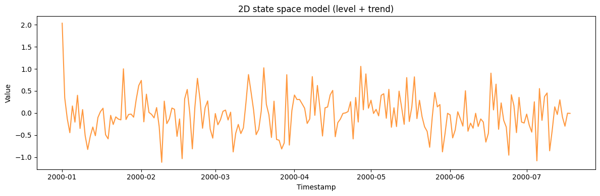
2. 2D state space model (level + trend)
A two-dimensional state captures both the level and its trend (rate of change).two_dim_params = {
"min_length": 200,
"max_length": 200,
"freq": "D",
"state_dim": 2,
"obs_dim": 1,
"seed": 42,
}
two_dim_gen = StateSpaceGenerator(engine="polars", **two_dim_params)
two_dim_df = two_dim_gen.generate(n_series=1)
print(f"Generated {len(two_dim_df)} observations from 2D state space model")
print(
f"Statistics: Mean={two_dim_df['y'].mean():.4f}, "
f"Std={two_dim_df['y'].std():.4f}"
)
two_dim_df.head(10)
Generated 200 observations from 2D state space model
Statistics: Mean=-0.0315, Std=0.4513
| unique_id | ds | y |
|---|---|---|
| cat | datetime[ns] | f64 |
| ”0” | 2000-01-01 00:00:00 | 2.035213 |
| ”0” | 2000-01-02 00:00:00 | 0.342724 |
| ”0” | 2000-01-03 00:00:00 | -0.130302 |
| ”0” | 2000-01-04 00:00:00 | -0.445831 |
| ”0” | 2000-01-05 00:00:00 | 0.159239 |
| ”0” | 2000-01-06 00:00:00 | -0.206335 |
| ”0” | 2000-01-07 00:00:00 | 0.401635 |
| ”0” | 2000-01-08 00:00:00 | -0.350341 |
| ”0” | 2000-01-09 00:00:00 | 0.077724 |
| ”0” | 2000-01-10 00:00:00 | -0.512018 |
fig, ax = plt.subplots(figsize=(12, 4))
ax.plot(two_dim_df["ds"].to_list(), two_dim_df["y"].to_list(), alpha=0.8, color="C1")
ax.set_xlabel("Timestamp")
ax.set_ylabel("Value")
ax.set_title("2D state space model (level + trend)")
plt.tight_layout()
plt.show()
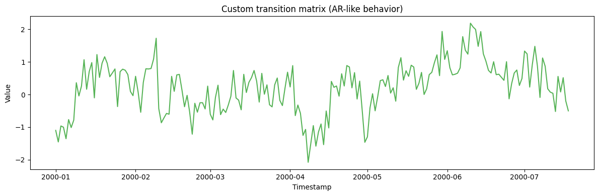
3. Custom transition matrix (AR-like behavior)
Specify a custom state transition matrix to create AR-like dynamics in the hidden state.transition_matrix = np.array([[0.9, 0.1], [0.0, 0.8]])
custom_transition_params = {
"min_length": 200,
"max_length": 200,
"freq": "D",
"state_dim": 2,
"obs_dim": 1,
"transition_matrix": transition_matrix.tolist(),
"seed": 42,
}
custom_transition_gen = StateSpaceGenerator(engine="polars", **custom_transition_params)
custom_transition_df = custom_transition_gen.generate(n_series=1)
print(f"Generated {len(custom_transition_df)} observations with custom transition matrix")
print(
f"Statistics: Mean={custom_transition_df['y'].mean():.4f}, "
f"Std={custom_transition_df['y'].std():.4f}"
)
custom_transition_df.head(10)
Generated 200 observations with custom transition matrix
Statistics: Mean=0.2258, Std=0.7764
| unique_id | ds | y |
|---|---|---|
| cat | datetime[ns] | f64 |
| ”0” | 2000-01-01 00:00:00 | -1.099579 |
| ”0” | 2000-01-02 00:00:00 | -1.454542 |
| ”0” | 2000-01-03 00:00:00 | -0.964621 |
| ”0” | 2000-01-04 00:00:00 | -1.002322 |
| ”0” | 2000-01-05 00:00:00 | -1.355461 |
| ”0” | 2000-01-06 00:00:00 | -0.768567 |
| ”0” | 2000-01-07 00:00:00 | -1.013438 |
| ”0” | 2000-01-08 00:00:00 | -0.786117 |
| ”0” | 2000-01-09 00:00:00 | 0.361217 |
| ”0” | 2000-01-10 00:00:00 | -0.043312 |
fig, ax = plt.subplots(figsize=(12, 4))
ax.plot(custom_transition_df["ds"].to_list(), custom_transition_df["y"].to_list(), alpha=0.8, color="C2")
ax.set_xlabel("Timestamp")
ax.set_ylabel("Value")
ax.set_title("Custom transition matrix (AR-like behavior)")
plt.tight_layout()
plt.show()
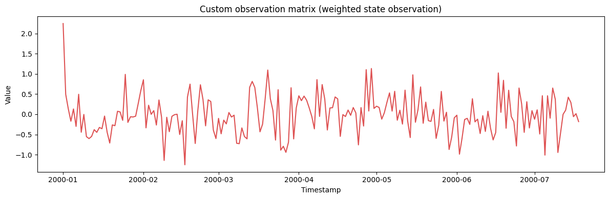
4. Custom observation matrix (weighted state observation)
Observe a weighted combination of the hidden states.observation_matrix = np.array([[1.0, 0.5]])
custom_obs_params = {
"min_length": 200,
"max_length": 200,
"freq": "D",
"state_dim": 2,
"obs_dim": 1,
"observation_matrix": observation_matrix.tolist(),
"seed": 42,
}
custom_obs_gen = StateSpaceGenerator(engine="polars", **custom_obs_params)
custom_obs_df = custom_obs_gen.generate(n_series=1)
print(f"Generated {len(custom_obs_df)} observations with custom observation matrix")
print(
f"Statistics: Mean={custom_obs_df['y'].mean():.4f}, "
f"Std={custom_obs_df['y'].std():.4f}"
)
custom_obs_df.head(10)
Generated 200 observations with custom observation matrix
Statistics: Mean=-0.0163, Std=0.4940
| unique_id | ds | y |
|---|---|---|
| cat | datetime[ns] | f64 |
| ”0” | 2000-01-01 00:00:00 | 2.24795 |
| ”0” | 2000-01-02 00:00:00 | 0.496252 |
| ”0” | 2000-01-03 00:00:00 | 0.135206 |
| ”0” | 2000-01-04 00:00:00 | -0.172047 |
| ”0” | 2000-01-05 00:00:00 | 0.132115 |
| ”0” | 2000-01-06 00:00:00 | -0.300323 |
| ”0” | 2000-01-07 00:00:00 | 0.495517 |
| ”0” | 2000-01-08 00:00:00 | -0.444273 |
| ”0” | 2000-01-09 00:00:00 | -0.004085 |
| ”0” | 2000-01-10 00:00:00 | -0.554032 |
fig, ax = plt.subplots(figsize=(12, 4))
ax.plot(custom_obs_df["ds"].to_list(), custom_obs_df["y"].to_list(), alpha=0.8, color="C3")
ax.set_xlabel("Timestamp")
ax.set_ylabel("Value")
ax.set_title("Custom observation matrix (weighted state observation)")
plt.tight_layout()
plt.show()
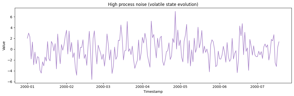
5. High process noise (volatile state evolution)
Increase the process noise covariance to create more volatile hidden state dynamics.high_process_noise = np.array([[5.0, 0.0], [0.0, 5.0]])
high_noise_params = {
"min_length": 200,
"max_length": 200,
"freq": "D",
"state_dim": 2,
"obs_dim": 1,
"state_covariance": high_process_noise.tolist(),
"seed": 42,
}
high_noise_gen = StateSpaceGenerator(engine="polars", **high_noise_params)
high_noise_df = high_noise_gen.generate(n_series=1)
print(f"Generated {len(high_noise_df)} observations with high process noise")
print(
f"Statistics: Mean={high_noise_df['y'].mean():.4f}, "
f"Std={high_noise_df['y'].std():.4f}"
)
high_noise_df.head(10)
Generated 200 observations with high process noise
Statistics: Mean=-0.1518, Std=2.2105
| unique_id | ds | y |
|---|---|---|
| cat | datetime[ns] | f64 |
| ”0” | 2000-01-01 00:00:00 | 2.035213 |
| ”0” | 2000-01-02 00:00:00 | 2.980453 |
| ”0” | 2000-01-03 00:00:00 | 2.307622 |
| ”0” | 2000-01-04 00:00:00 | -1.815772 |
| ”0” | 2000-01-05 00:00:00 | 1.32836 |
| ”0” | 2000-01-06 00:00:00 | -2.890637 |
| ”0” | 2000-01-07 00:00:00 | -0.526938 |
| ”0” | 2000-01-08 00:00:00 | -2.710086 |
| ”0” | 2000-01-09 00:00:00 | -1.37662 |
| ”0” | 2000-01-10 00:00:00 | -1.535066 |
fig, ax = plt.subplots(figsize=(12, 4))
ax.plot(high_noise_df["ds"].to_list(), high_noise_df["y"].to_list(), alpha=0.8, color="C4")
ax.set_xlabel("Timestamp")
ax.set_ylabel("Value")
ax.set_title("High process noise (volatile state evolution)")
plt.tight_layout()
plt.show()
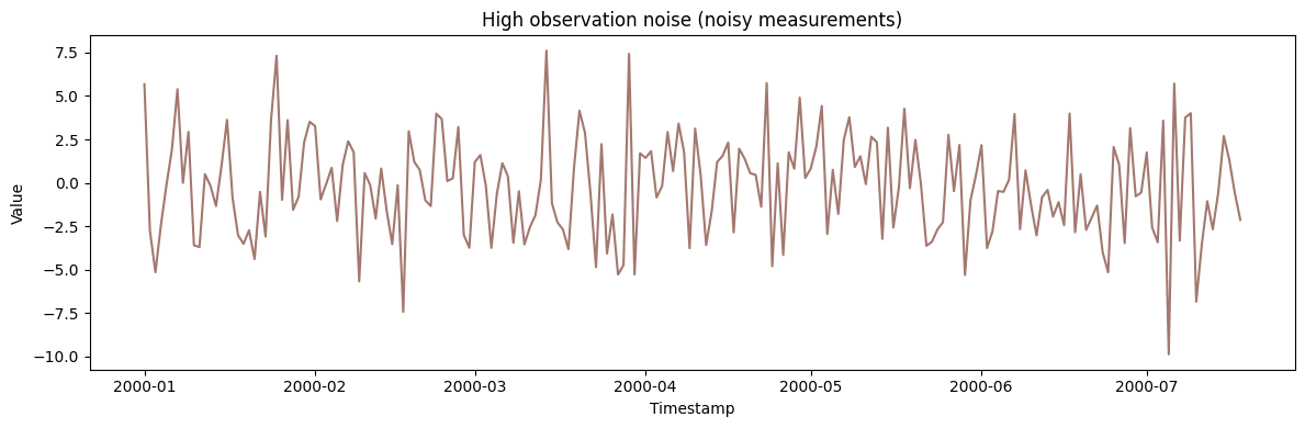
6. High observation noise (noisy measurements)
Increase the observation noise to simulate noisy measurement conditions.high_obs_noise = np.array([[10.0]])
noisy_obs_params = {
"min_length": 200,
"max_length": 200,
"freq": "D",
"state_dim": 2,
"obs_dim": 1,
"obs_covariance": high_obs_noise.tolist(),
"seed": 42,
}
noisy_obs_gen = StateSpaceGenerator(engine="polars", **noisy_obs_params)
noisy_obs_df = noisy_obs_gen.generate(n_series=1)
print(f"Generated {len(noisy_obs_df)} observations with high observation noise")
print(
f"Statistics: Mean={noisy_obs_df['y'].mean():.4f}, "
f"Std={noisy_obs_df['y'].std():.4f}"
)
noisy_obs_df.head(10)
Generated 200 observations with high observation noise
Statistics: Mean=-0.2227, Std=2.9604
| unique_id | ds | y |
|---|---|---|
| cat | datetime[ns] | f64 |
| ”0” | 2000-01-01 00:00:00 | 5.679936 |
| ”0” | 2000-01-02 00:00:00 | -2.754326 |
| ”0” | 2000-01-03 00:00:00 | -5.158032 |
| ”0” | 2000-01-04 00:00:00 | -2.433461 |
| ”0” | 2000-01-05 00:00:00 | -0.135867 |
| ”0” | 2000-01-06 00:00:00 | 1.917522 |
| ”0” | 2000-01-07 00:00:00 | 5.393208 |
| ”0” | 2000-01-08 00:00:00 | -0.005179 |
| ”0” | 2000-01-09 00:00:00 | 2.933222 |
| ”0” | 2000-01-10 00:00:00 | -3.603567 |
fig, ax = plt.subplots(figsize=(12, 4))
ax.plot(noisy_obs_df["ds"].to_list(), noisy_obs_df["y"].to_list(), alpha=0.8, color="C5")
ax.set_xlabel("Timestamp")
ax.set_ylabel("Value")
ax.set_title("High observation noise (noisy measurements)")
plt.tight_layout()
plt.show()
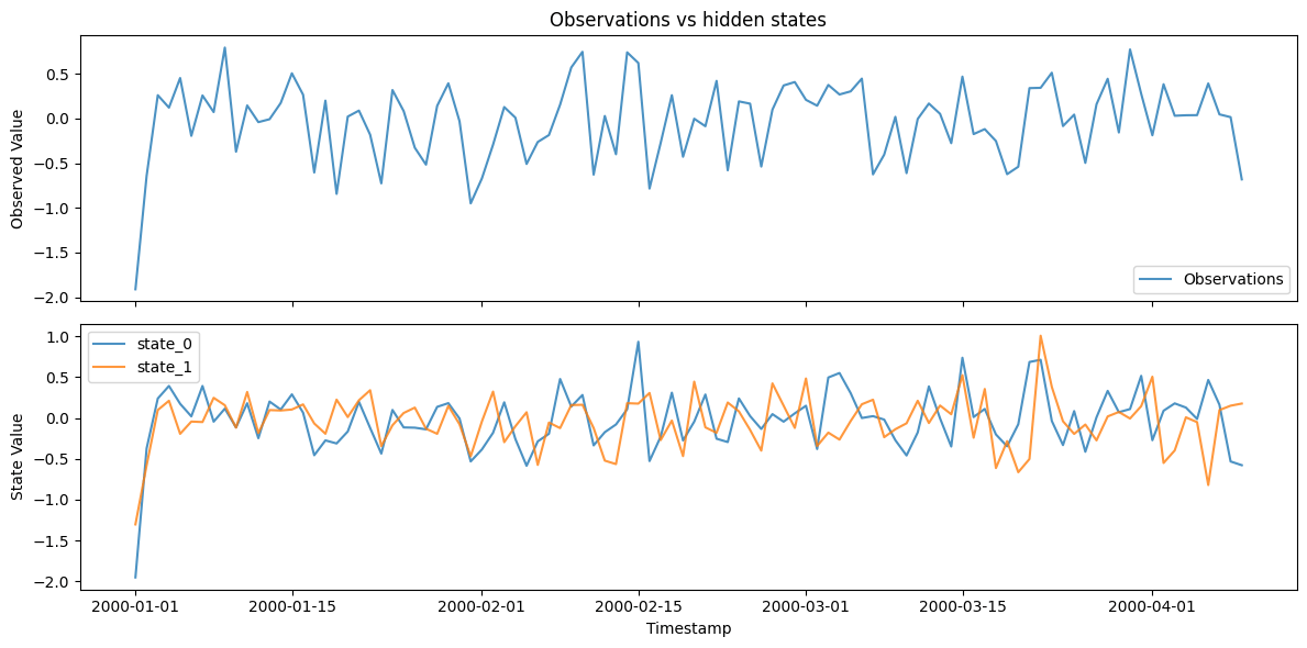
7. Generate with hidden states
Return both observations and hidden states to inspect the latent dynamics.with_states_params = {
"min_length": 100,
"max_length": 100,
"freq": "D",
"state_dim": 2,
"obs_dim": 1,
"seed": 42,
}
with_states_gen = StateSpaceGenerator(engine="polars", **with_states_params)
obs_df, states_df = with_states_gen.generate_with_states(n_series=1)
print(f"Generated observations and hidden states")
print(
f"Observation Statistics: Mean={obs_df['y'].mean():.4f}, "
f"Std={obs_df['y'].std():.4f}"
)
print("\nObservations:")
print(obs_df.head(10))
print("\nHidden States:")
print(states_df.head(10))
Generated observations and hidden states
Observation Statistics: Mean=-0.0286, Std=0.4412

Observations:
shape: (10, 3)
┌───────────┬─────────────────────┬───────────┐
│ unique_id ┆ ds                  ┆ y         │
│ ---       ┆ ---                 ┆ ---       │
│ cat       ┆ datetime[ns]        ┆ f64       │
╞═══════════╪═════════════════════╪═══════════╡
│ 0         ┆ 2000-01-01 00:00:00 ┆ -1.910609 │
│ 0         ┆ 2000-01-02 00:00:00 ┆ -0.642705 │
│ 0         ┆ 2000-01-03 00:00:00 ┆ 0.258913  │
│ 0         ┆ 2000-01-04 00:00:00 ┆ 0.120297  │
│ 0         ┆ 2000-01-05 00:00:00 ┆ 0.451117  │
│ 0         ┆ 2000-01-06 00:00:00 ┆ -0.195514 │
│ 0         ┆ 2000-01-07 00:00:00 ┆ 0.256028  │
│ 0         ┆ 2000-01-08 00:00:00 ┆ 0.070385  │
│ 0         ┆ 2000-01-09 00:00:00 ┆ 0.791294  │
│ 0         ┆ 2000-01-10 00:00:00 ┆ -0.372822 │
└───────────┴─────────────────────┴───────────┘

Hidden States:
shape: (10, 4)
┌───────────┬─────────────────────┬───────────┬───────────┐
│ unique_id ┆ ds                  ┆ state_0   ┆ state_1   │
│ ---       ┆ ---                 ┆ ---       ┆ ---       │
│ cat       ┆ datetime[ns]        ┆ f64       ┆ f64       │
╞═══════════╪═════════════════════╪═══════════╪═══════════╡
│ 0         ┆ 2000-01-01 00:00:00 ┆ -1.951035 ┆ -1.30218  │
│ 0         ┆ 2000-01-02 00:00:00 ┆ -0.372949 ┆ -0.5793   │
│ 0         ┆ 2000-01-03 00:00:00 ┆ 0.238032  ┆ 0.097115  │
│ 0         ┆ 2000-01-04 00:00:00 ┆ 0.39203   ┆ 0.210554  │
│ 0         ┆ 2000-01-05 00:00:00 ┆ 0.173327  ┆ -0.193943 │
│ 0         ┆ 2000-01-06 00:00:00 ┆ 0.019815  ┆ -0.044133 │
│ 0         ┆ 2000-01-07 00:00:00 ┆ 0.391477  ┆ -0.049829 │
│ 0         ┆ 2000-01-08 00:00:00 ┆ -0.045179 ┆ 0.24666   │
│ 0         ┆ 2000-01-09 00:00:00 ┆ 0.114046  ┆ 0.155727  │
│ 0         ┆ 2000-01-10 00:00:00 ┆ -0.115485 ┆ -0.119006 │
└───────────┴─────────────────────┴───────────┴───────────┘
fig, axes = plt.subplots(2, 1, figsize=(12, 6), sharex=True)
axes[0].plot(obs_df["ds"].to_list(), obs_df["y"].to_list(), alpha=0.8, label="Observations")
axes[0].set_ylabel("Observed Value")
axes[0].set_title("Observations vs hidden states")
axes[0].legend()

state_cols = [c for c in states_df.columns if c.startswith("state_")]
for col in state_cols:
    axes[1].plot(states_df["ds"].to_list(), states_df[col].to_list(), alpha=0.8, label=col)
axes[1].set_xlabel("Timestamp")
axes[1].set_ylabel("State Value")
axes[1].legend()
plt.tight_layout()
plt.show()
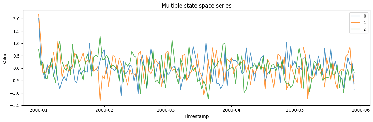
8. Multiple state space series
Generate multiple independent state space series.multi_params = {
"min_length": 150,
"max_length": 150,
"freq": "D",
"state_dim": 2,
"obs_dim": 1,
"seed": 42,
}
multi_gen = StateSpaceGenerator(engine="polars", **multi_params)
multi_df = multi_gen.generate(n_series=3)
print(f"Generated 3 series with {len(multi_df)} total observations")
print(
f"Overall Statistics: Mean={multi_df['y'].mean():.4f}, "
f"Std={multi_df['y'].std():.4f}"
)
multi_df.filter(pl.col("unique_id") == "0").head(10)
Generated 3 series with 450 total observations
Overall Statistics: Mean=-0.0026, Std=0.4818
| unique_id | ds | y |
|---|---|---|
| cat | datetime[ns] | f64 |
| ”0” | 2000-01-01 00:00:00 | 2.035213 |
| ”0” | 2000-01-02 00:00:00 | 0.342724 |
| ”0” | 2000-01-03 00:00:00 | -0.130302 |
| ”0” | 2000-01-04 00:00:00 | -0.445831 |
| ”0” | 2000-01-05 00:00:00 | 0.159239 |
| ”0” | 2000-01-06 00:00:00 | -0.206335 |
| ”0” | 2000-01-07 00:00:00 | 0.401635 |
| ”0” | 2000-01-08 00:00:00 | -0.350341 |
| ”0” | 2000-01-09 00:00:00 | 0.077724 |
| ”0” | 2000-01-10 00:00:00 | -0.512018 |
fig, ax = plt.subplots(figsize=(12, 4))
for uid in multi_df["unique_id"].unique().to_list():
    series = multi_df.filter(pl.col("unique_id") == uid)
    ax.plot(series["ds"].to_list(), series["y"].to_list(), label=uid, alpha=0.8)
ax.set_xlabel("Timestamp")
ax.set_ylabel("Value")
ax.set_title("Multiple state space series")
ax.legend()
plt.tight_layout()
plt.show()
Related generatorsFull parameters are in the generator reference.
- SARIMA and ETS — specific state-space families.
- Chaotic system — deterministic nonlinear dynamics.