

Summary
- Twelve native features (
native_v1) are defined for every one of the 100,000 M4 training series under declared period and window recipes, and they respond in the expected direction to controlled changes in dependence, seasonality, spikes, level shifts, and variance shifts.- M4, Yearly to Daily: the interpretable and pretraining pools cover 52–88% of fresh held-out real queries at the real-calibrated radius, against real-to-real baselines of 80–91%. No M4 panel other than Hourly shows a material gap over three generation seeds and four query groups.
- M4 Hourly is the largest gap: 1–2% coverage against a 91% baseline, replicated on 288 distinct real queries. The missing combination is a daily cycle with slow level and amplitude changes; trend strength alone carries about half the remaining distance.
- Independent panels change the picture: on Monash tourism quarterly and Australian weather daily the pools also fall 35 points or more short, and hospital monthly is 27 points short, while tourism yearly and traffic weekly are covered as well as M4. Gaps are panel-specific, with strong regular seasonality the recurring theme.
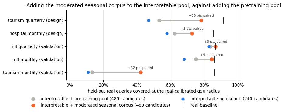
- Configuring existing generators closes most of the M4 Hourly gap (67% coverage) but transfers only partly to an independent traffic panel (19%). A moderated seasonal corpus, added to the interpretable pool at equal candidate count, raises coverage on all five quarterly and monthly panels tested, three of them held out, by 3 to 32 points. That corpus ships as the opt-in
seasonal_pool()preset; a pre-declared test on four more panels passes on M1 monthly, is neutral on M4, and shows no benefit on intermittent data, so the default pools are unchanged.
What is measured
compute_features returns one row of twelve summaries per series:
spectral entropy, trend and seasonal strength from a classical
decomposition, four autocorrelation summaries, spike and lumpiness, the
largest level and variance shift between adjacent windows, and the
number of median crossings. The definitions are frozen as native_v1;
the seasonal period and window width are extraction parameters that you
declare per panel, not part of the schema.
The example below extracts features for a small hourly panel and
compares two synthetic sources in that space with
compare_feature_coverage. It needs no network access, so the reference
here is itself synthetic; the benchmarks further down use real M4 and
traffic data.
CoverageResult reports which features were used, how many series
each side retained, and grid-based miscoverage in a two-dimensional PCA
map fitted on the reference alone. The map is a convenient picture, but
two dimensions keep only 54–84% of the feature variance on M4 panels, so
the benchmarks score coverage on all standardized features and use
the map only for illustration.
How the benchmarks score coverageQueries are always disjoint from the fitting and calibration series, criteria are declared before results are inspected, and repeated settings use fresh queries rather than the ones that informed a design. Coverage is conditional on the twelve features, the distance, and the radius; Manhattan distance and single-feature omissions are reported as sensitivity checks.
- Fit the feature mean and scale on 64 real reference series only. Synthetic data never shifts the space.
- For each held-out real query, find its nearest synthetic series and its nearest real candidate in standardized Euclidean distance.
- Calibrate a radius as the 90th percentile of nearest distances from 32 separate real calibration queries to the real candidates.
- Coverage is the fraction of queries whose nearest synthetic series lies within that radius. The real baseline is the same fraction using real candidates, and bounds what any corpus of that size can reach.
- Synthetic and real candidates are matched one-to-one in count and length, so candidate density cannot favour either side.
Coverage across frequencies
The cross-frequency benchmark samples 640 training series per M4 frequency (all 359 for Weekly), forms four disjoint groups of 64 fresh queries, and scores the unchangedinterpretable_pool (stored under the
key balanced_pool in the benchmark artifacts, its name at the time),
pretraining_pool, and a random MAR corpus over three generation seeds
with 240 matched candidates each. Hourly comes from the earlier
fresh-split validation, which used the same protocol.
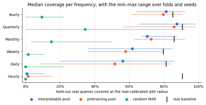
- Yearly and Quarterly are essentially covered. The pools sit within a few points of what real candidates achieve. Monthly falls about 5 points short and Weekly about 20, the latter flagged as a minor gap. Daily is the widest of the three, roughly 25 to 30 points below the real-to-real baseline, and depends strongly on which real series are queried (two folds gap by more than 25 points, two by less than 10).
- The two pools are interchangeable here. They stay within five points of each other on every panel, so the meta-generators added by the pretraining pool do not buy coverage in this feature space. Random MAR is far behind on every panel, Quarterly included, where it reaches 34% against 88% for the pools.
- Hourly is a different regime. Coverage is 1–2% against a 91% baseline, and the twelve fold–seed pairs never exceed 16%. The rest of this page is about that gap.
What covered queries look like
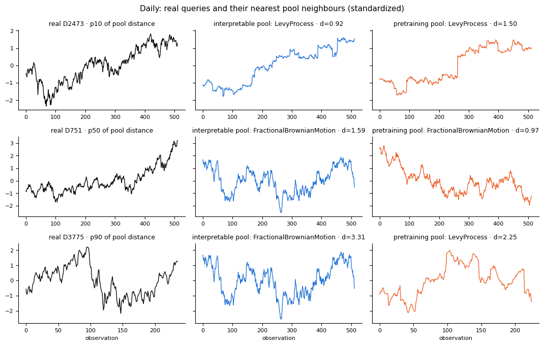
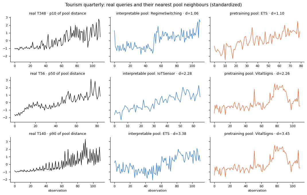
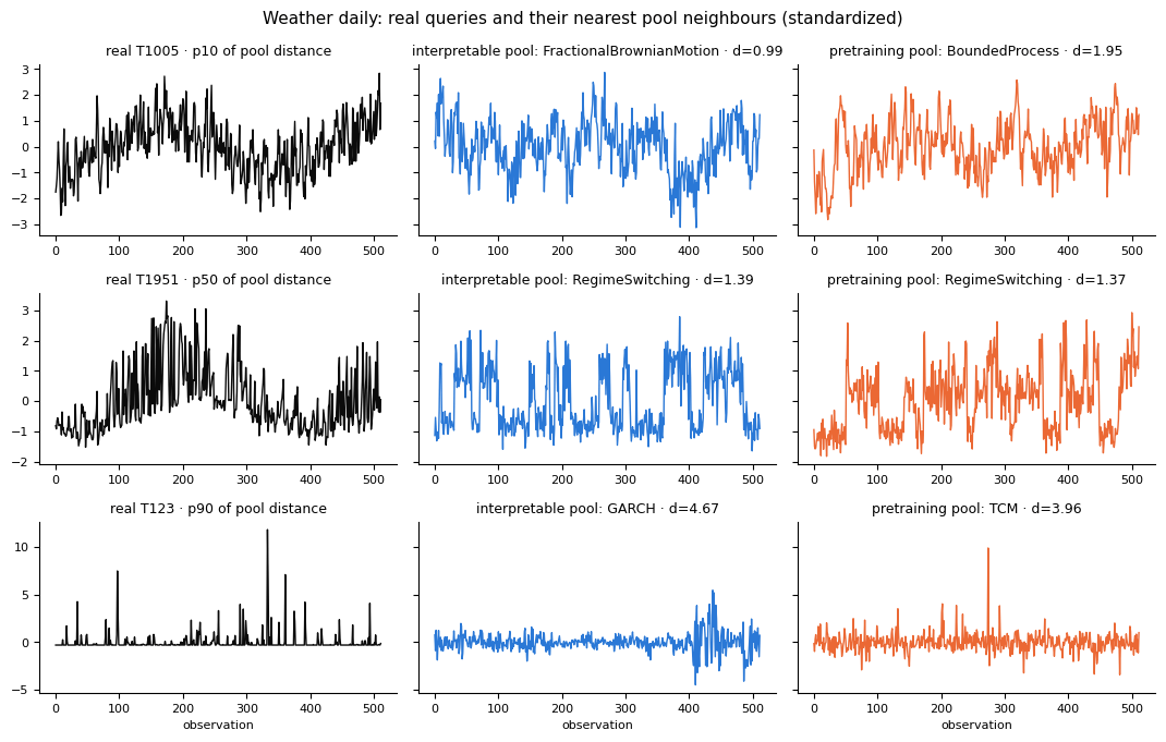
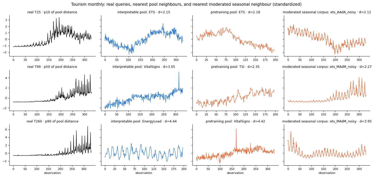
Coverage numbers summarize distances between feature vectors, so it is worth checking that a covered query actually resembles its nearest synthetic neighbour. The examples below are real M4 series from the first fold and first seed of the benchmark above, chosen at fixed rank percentiles (10th, 50th, 90th) of their distance to the interpretable pool rather than for visual effect, and shown next to their nearest neighbour from each pool. Every series is standardized so that shape, not scale, is compared; the label gives the generator prototype and the standardized feature distance.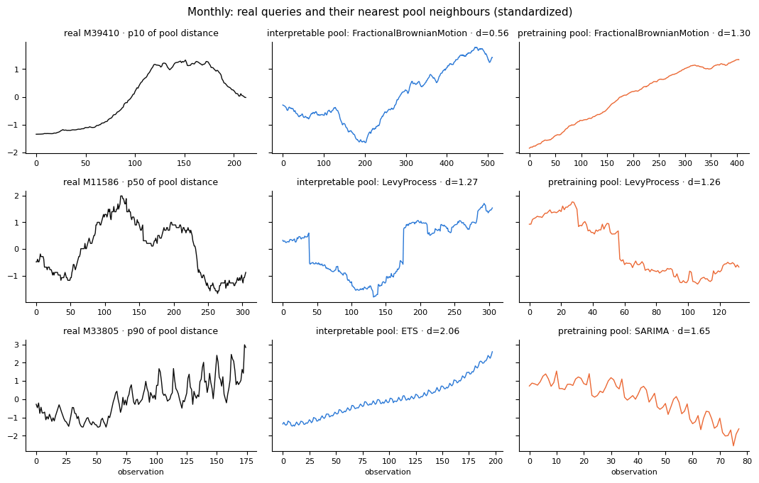
Independent panels
M4 is one source, so each non-hourly frequency was also scored on a public Monash panel from another domain with the identical protocol: tourism demand (yearly and quarterly), hospital patient counts (monthly), San Francisco freeway occupancy (weekly), and Australian weather stations (daily). Hourly’s independent panel is the traffic dataset used in the composition rounds below.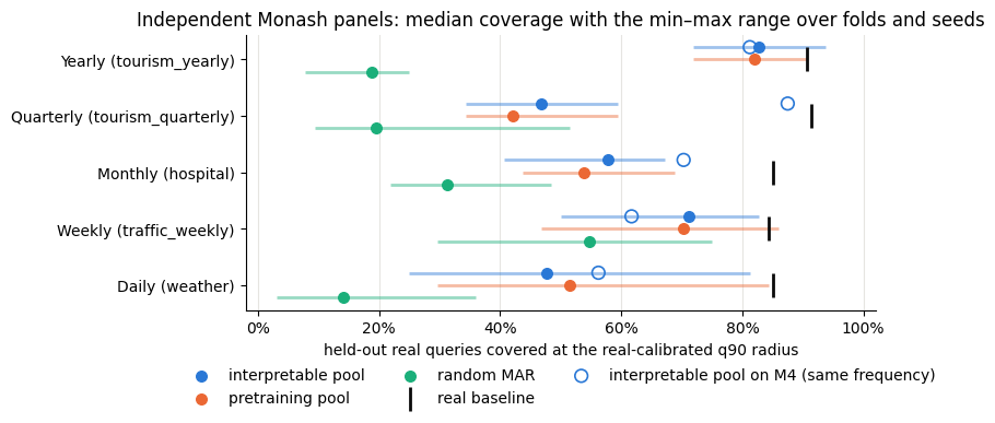
The Hourly gap
The Hourly result was replicated on fixed queries with ten fresh generation seeds and four times more candidates, then on 256 additional queries in four disjoint groups. Neither more draws nor more candidates closed it. Decomposing the nearest-neighbour distances shows that trend strength contributes about half of the mean squared distance: real hourly series have far stronger trend components than their nearest synthetic neighbours, whose daily cycles sit on a flat level. Omitting trend strength from the distance raises pool coverage to about 44%, so the gap is not only trend, but trend is where it starts. To test that reading, paired diagnostic controls were generated from a unit daily sine plus noise, adding one component at a time: a slow level drift, a weekly amplitude envelope, and a second daily harmonic. The controls use no real values and share their random components within each slot, so each row below differs from the previous one by exactly one ingredient.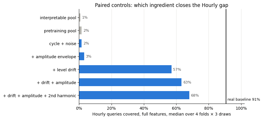
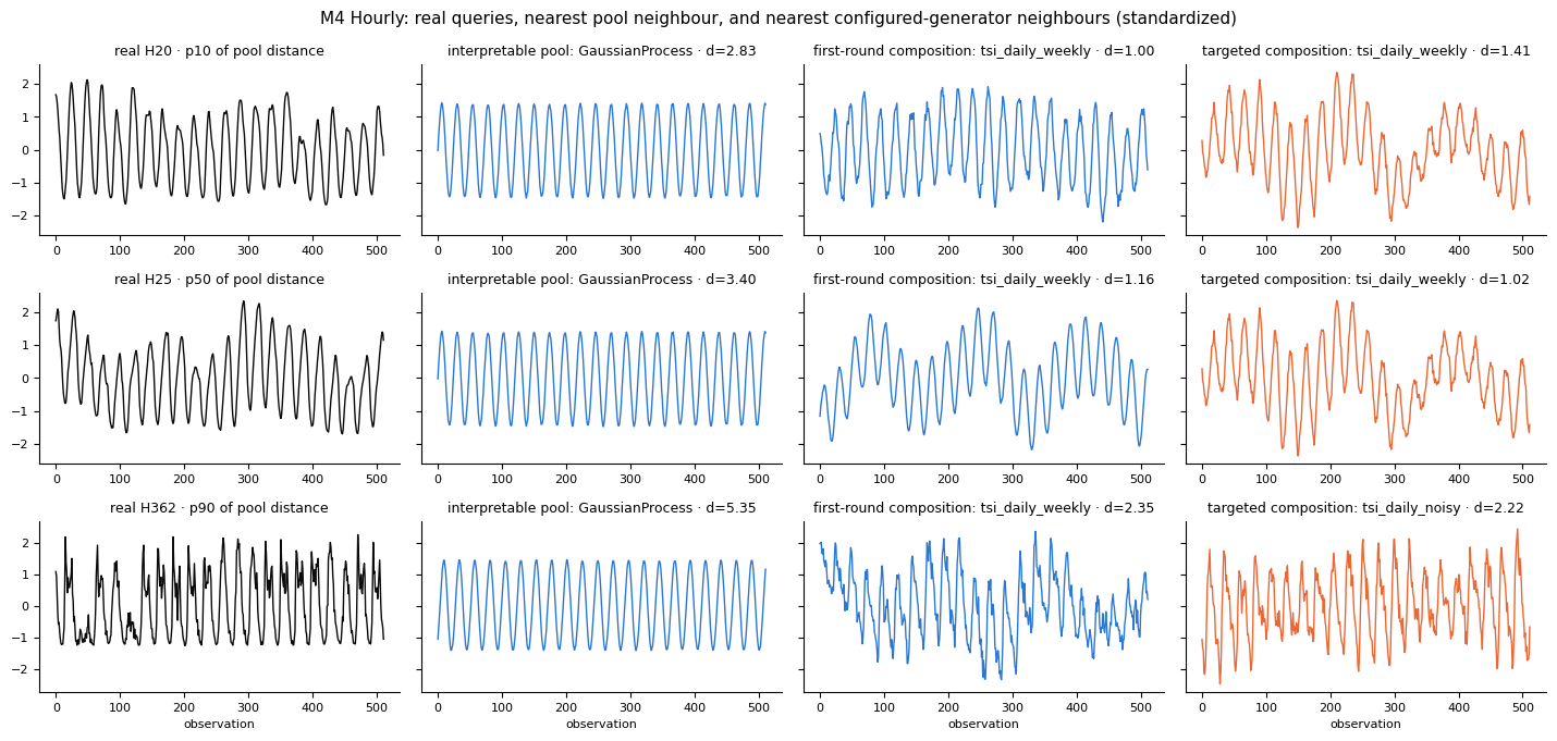
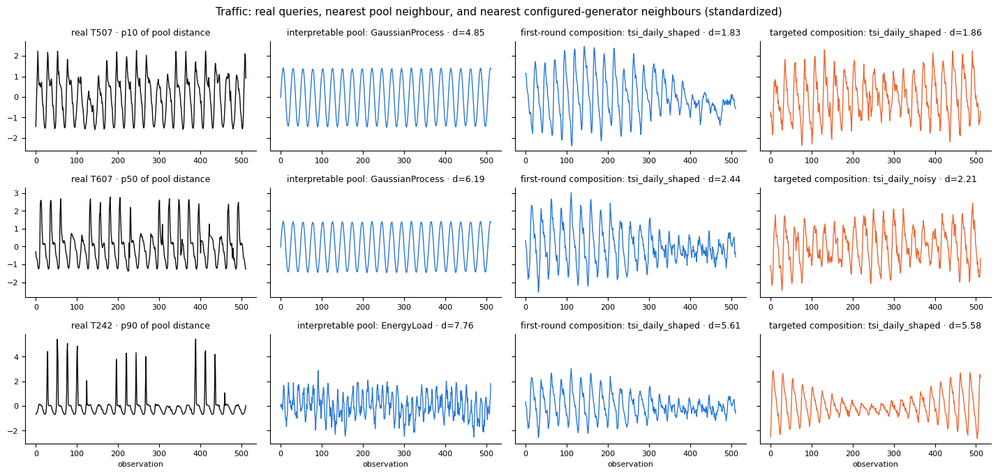
TSIGenerator prototype, and its neighbours
share the real series’ slow variation; the targeted round’s noisier
variant picks up the jagged query. The standardized feature distances
fall from 2.8–5.4 for the pool to 1.0–2.4 for the compositions. The
daily shapes remain smoother than the real ones, which is the
daily-profile score the compositions did not improve.
Can existing generators close it?
The controls are diagnostic recipes, not generators. The next question was whether the shipped classes can express the same combination through configuration alone. A benchmark-only corpus of eight prototypes was declared before inspection:TSIGenerator restricted to a period-24
harmonic with overtones, a slow amplitude envelope, and a drifting
trend; ETSGenerator with multiplicative period-24 seasonality on a
random-walk level; SeasonalGenerator with injected slope and level
changepoints; and EnergyLoadGenerator profiles with a slope change. It
was scored on the same fresh M4 splits and then on 862 hourly traffic
series from the Monash repository, a panel that had not informed the
design. A second, targeted round then added noisier and level-shifting
variants and was scored on traffic queries never used before, with M4
kept as a retention check.
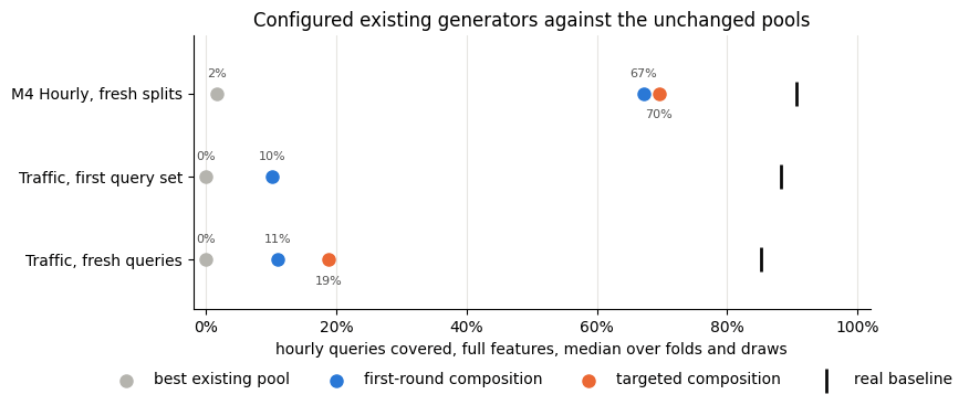
TSIGenerator prototypes supply three quarters of the nearest
neighbours; the ETSGenerator prototypes are never nearest. It does not
reproduce the controls’ improvement in average daily shape.
On traffic the same corpus improves coverage in every paired comparison
but only to about 10%, and the targeted second round roughly doubles
that to 19% on queries never used before, while keeping the M4 result.
Both rounds fall short of the declared threshold of a 25-point median
gain over the best pool in three of four folds. The remaining traffic
distance concerns crossing points and ten-lag autocorrelation: real
traffic series combine low within-day autocorrelation with long
excursions on one side of the mean, which none of the configured
generators produce together.
Can configuration close the seasonal gaps?
The same approach was applied to the seasonal theme. Two benchmark-only corpora of configuredTSIGenerator, ETSGenerator, and
SeasonalGenerator instances at the panel period were scored on the two
panels that motivated them, tourism quarterly and hospital monthly, and
then on three panels that did not: M3 quarterly, M3 monthly, and tourism
monthly. The first recipe was declared before any result and aimed at
strong seasonality; it turned out far too clean, with seasonal strength
near one and almost no noise, while the real series sit at moderate
seasonal strength under heavy noise. The second, moderated recipe was
declared after that diagnosis on the design panels only, and nothing was
changed once the validation panels were scored.
The shipped preset and its pre-declared test
The moderated corpus now ships as the opt-inseasonal_pool() preset,
with exactly the configuration benchmarked above. Because the augmented
comparison had been chosen after the fact, it was declared as the
criterion before testing the preset on four panels never used in any
earlier step: fresh M4 Quarterly and Monthly samples, M1 monthly, and
intermittent car-parts sales as a no-harm check. The gates were a median
paired gain of at least 5 points in three of four folds, and no fold
below −2 points, for interpretable + preset against interpretable +
pretraining at 480 candidates each.
The verdict is mixed and is reported as such. M1 monthly, where the
pools sit 24 points below the real baseline, passes both gates with a
12.5-point paired gain and is the only clear pass. The two fresh M4
samples have no seasonal gap to fill and come out neutral, though M4
Quarterly misses the no-harm gate by one point in one fold. Car parts
fails no-harm: its gap is an intermittent-demand gap that the seasonal
preset does not address, while the pretraining pool’s meta-generators
help a little, so displacing their share costs 3 points. Added on top of
both pools rather than in place of a share, a post-hoc comparison
against adding random MAR shows the preset helps where seasonality is
strong and is within a point either way elsewhere, including −0.8 points
on car parts. That is how the preset is documented: an opt-in addition
on top of a pool, kept out of the defaults.
A last pre-declared test asked whether the addition should become the
pretraining_pool default, through the new include_seasonal flag, by
comparing the pool with and without it as equal-count corpora on fifteen
panels at every frequency but yearly. The flag raised coverage on every
quarterly and monthly panel, by 2 to 14 points, and lowered it on
weekly, daily, and intermittent panels, by up to about 6 points on M4
weekly and daily and about 3 on car parts, while traffic weekly and
weather daily were essentially unchanged; it builds a cycle those series
do not have and displaces breadth. Six panels failed the no-harm gate,
so the default stays off, and the flag is recommended for quarterly and
monthly targets only. The table below is from that run.
What this means for the presets
Recommendation
- Keep the production pools as they are for now. The two pools are interchangeable for coverage, and no single configuration has yet been shown to close a gap on a panel that did not inform it, so there is no evidence-backed change to
interpretable_poolorpretraining_pooldefaults.- The gap is about strong regular seasonality on a moving level, not one frequency. Within M4 only Hourly is short, but tourism quarterly and monthly, hospital monthly, and weather daily are also under-covered on independent panels.
- Ship gap-filling corpora as opt-in additions, not replacements.
seasonal_pool()is now available for that purpose: it raised coverage on tourism, hospital, and M1 monthly panels, was neutral on M4, and gave nothing on intermittent data, so it belongs on top of a pool and outside the defaults. A comparable hourly preset would need the same pre-declared test on a third hourly panel first.- Evaluate on held-out panels, not M4 alone. M4 Quarterly looked covered at 88% while tourism quarterly is at 47%; a benchmark on one source can miss a gap that another source shows.
What coverage does not tell you
- Coverage is conditional on the twelve
native_v1features, standardized Euclidean distance, a q90 radius, and the declared period and window per panel. Manhattan distance and feature omissions shift absolute levels by up to ten points, and by far more on Hourly.- Fold–seed measurements share real series across roles and are not independent replications; there are no confidence intervals in these summaries.
- A covered query has a synthetic neighbour with similar summaries, not a similar series. Nothing here measures forecasting accuracy, raw-series distance, or privacy.
Reproduce
The benchmark scripts and their artifacts are not yet in the repository; they land in a follow-up pull request that keeps this one focused on the library change. The commands below are recorded now so the protocol is on the record, and the numbers on this page come from a local run of exactly these steps. Once the scripts land they run in sequence, each reading the previous one’ssummary.json, with detailed per-query
traces written alongside and a README per directory documenting
protocol, results, and limits.
benchmarks/data/feature_coverage_*/, which
is untracked. The API used above, compute_features and
compare_feature_coverage, is documented in the evaluation
reference.