> ## Documentation Index
> Fetch the complete documentation index at: https://nixtlaverse.nixtla.io/llms.txt
> Use this file to discover all available pages before exploring further.
# Hawkes process (self-excitation)
A Hawkes process is a *self-exciting* arrival process: each event
temporarily raises the probability of further events, producing the
clustered bursts seen in trades, earthquakes, and social-media cascades.
It is the natural counterpoint to the memoryless Poisson process.
> **The model**
>
> $\lambda(t) = \mu + \sum_{t_i \le t} g(t - t_i), \qquad g(t) = \alpha e^{-\beta t}$
>
> The arrival intensity is a baseline rate plus a decaying kick after
> every event, so activity begets activity. The excitation strength and
> decay set how tightly events cluster and how long a burst lasts; below
> a stability threshold the process stays finite.
```python theme={null}
import polars as pl
import matplotlib.pyplot as plt
from synforecast.generators import HawkesProcessGenerator
```
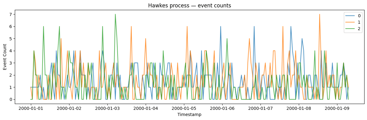
## 1. Event counts (default output)
Generate event count time series with a baseline intensity and
self-excitation.
```python theme={null}
params = {
"min_length": 200,
"max_length": 200,
"freq": "h",
"baseline_intensity": 1.0,
"excitation_amplitude": 0.5,
"decay_rate": 2.0,
"output_type": "counts",
"seed": 42,
}
generator = HawkesProcessGenerator(engine="polars", **params)
df = generator.generate(n_series=3)
print(f"Generated {df['unique_id'].n_unique()} time series")
print(f"Total observations: {len(df)}")
print(f"Total events: {df['y'].sum()}")
stats = df.group_by("unique_id").agg(
[
pl.col("y").sum().alias("total_events"),
pl.col("y").mean().alias("mean_per_hour"),
pl.col("y").max().alias("max_in_hour"),
]
)
stats
```
```text theme={null}
Generated 3 time series
Total observations: 600
Total events: 836.0
```
| unique\_id | total\_events | mean\_per\_hour | max\_in\_hour |
| ---------- | ------------- | --------------- | ------------- |
| cat | f64 | f64 | f64 |
| "0" | 286.0 | 1.43 | 6.0 |
| "2" | 245.0 | 1.225 | 7.0 |
| "1" | 305.0 | 1.525 | 7.0 |
```python theme={null}
fig, ax = plt.subplots(figsize=(12, 4))
for uid in df["unique_id"].unique().to_list():
series = df.filter(pl.col("unique_id") == uid)
ax.plot(series["ds"].to_list(), series["y"].to_list(), label=uid, alpha=0.8)
ax.set_xlabel("Timestamp")
ax.set_ylabel("Event Count")
ax.set_title("Hawkes process — event counts")
ax.legend()
plt.tight_layout()
plt.show()
```
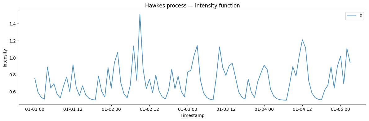
 ## 2. Intensity process
Output the underlying intensity function instead of event counts.
```python theme={null}
intensity_gen = HawkesProcessGenerator(engine="polars",
**{
"min_length": 100,
"max_length": 100,
"freq": "h",
"baseline_intensity": 0.5,
"excitation_amplitude": 0.3,
"decay_rate": 1.0,
"output_type": "intensity",
"seed": 42,
}
)
intensity_df = intensity_gen.generate(n_series=1)
print(f"Intensity range: [{intensity_df['y'].min():.3f}, {intensity_df['y'].max():.3f}]")
print(f"Mean intensity: {intensity_df['y'].mean():.3f}")
```
```text theme={null}
Intensity range: [0.501, 1.510]
Mean intensity: 0.723
```
```python theme={null}
fig, ax = plt.subplots(figsize=(12, 4))
for uid in intensity_df["unique_id"].unique().to_list():
series = intensity_df.filter(pl.col("unique_id") == uid)
ax.plot(series["ds"].to_list(), series["y"].to_list(), label=uid, alpha=0.8)
ax.set_xlabel("Timestamp")
ax.set_ylabel("Intensity")
ax.set_title("Hawkes process — intensity function")
ax.legend()
plt.tight_layout()
plt.show()
```
## 2. Intensity process
Output the underlying intensity function instead of event counts.
```python theme={null}
intensity_gen = HawkesProcessGenerator(engine="polars",
**{
"min_length": 100,
"max_length": 100,
"freq": "h",
"baseline_intensity": 0.5,
"excitation_amplitude": 0.3,
"decay_rate": 1.0,
"output_type": "intensity",
"seed": 42,
}
)
intensity_df = intensity_gen.generate(n_series=1)
print(f"Intensity range: [{intensity_df['y'].min():.3f}, {intensity_df['y'].max():.3f}]")
print(f"Mean intensity: {intensity_df['y'].mean():.3f}")
```
```text theme={null}
Intensity range: [0.501, 1.510]
Mean intensity: 0.723
```
```python theme={null}
fig, ax = plt.subplots(figsize=(12, 4))
for uid in intensity_df["unique_id"].unique().to_list():
series = intensity_df.filter(pl.col("unique_id") == uid)
ax.plot(series["ds"].to_list(), series["y"].to_list(), label=uid, alpha=0.8)
ax.set_xlabel("Timestamp")
ax.set_ylabel("Intensity")
ax.set_title("Hawkes process — intensity function")
ax.legend()
plt.tight_layout()
plt.show()
```
 ## 3. Model information and stability
Inspect model parameters including the branching ratio which determines
stability.
```python theme={null}
info = generator.get_model_info()
print(f"Baseline intensity (mu): {info['baseline_intensity']}")
print(f"Excitation amplitude (alpha): {info['excitation_amplitude']}")
print(f"Decay rate (beta): {info['decay_rate']}")
print(f"Branching ratio (alpha/beta): {info['branching_ratio']:.3f}")
print(f"Expected cluster size: {info['expected_cluster_size']:.3f}")
print(f"Process is stable: {info['is_stable']}")
```
```text theme={null}
Baseline intensity (mu): 1.0
Excitation amplitude (alpha): 0.5
Decay rate (beta): 2.0
Branching ratio (alpha/beta): 0.250
Expected cluster size: 1.333
Process is stable: True
```
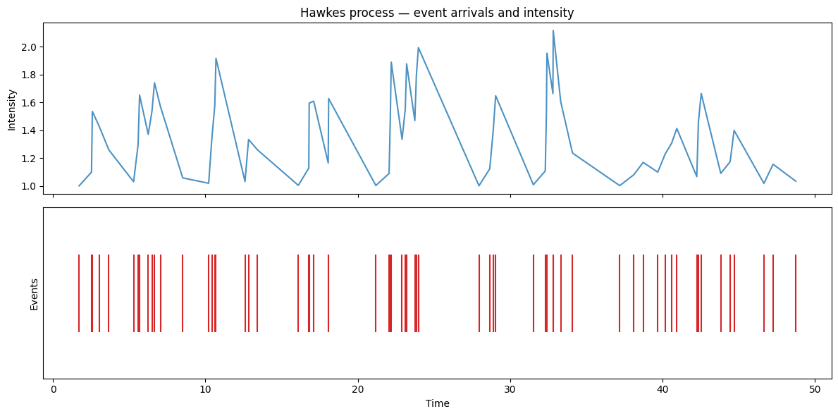
## 4. Raw event simulation
Directly simulate event arrival times and their associated intensities.
```python theme={null}
event_times, intensities = generator.simulate_with_events(time_horizon=50.0)
print(f"Simulated {len(event_times)} events over 50 time units")
print(f"Event rate: {len(event_times) / 50:.2f} events/unit time")
print(f"First 10 event times: {event_times[:10].round(3)}")
```
```text theme={null}
Simulated 64 events over 50 time units
Event rate: 1.28 events/unit time
First 10 event times: [1.714 2.527 2.584 3.022 3.662 5.29 5.583 5.682 6.25 6.494]
```
```python theme={null}
fig, axes = plt.subplots(2, 1, figsize=(12, 6), sharex=True)
axes[0].plot(event_times, intensities, alpha=0.8)
axes[0].set_ylabel("Intensity")
axes[0].set_title("Hawkes process — event arrivals and intensity")
axes[1].eventplot([event_times], lineoffsets=0.5, linelengths=0.8, colors="tab:red")
axes[1].set_xlabel("Time")
axes[1].set_ylabel("Events")
axes[1].set_yticks([])
plt.tight_layout()
plt.show()
```
## 3. Model information and stability
Inspect model parameters including the branching ratio which determines
stability.
```python theme={null}
info = generator.get_model_info()
print(f"Baseline intensity (mu): {info['baseline_intensity']}")
print(f"Excitation amplitude (alpha): {info['excitation_amplitude']}")
print(f"Decay rate (beta): {info['decay_rate']}")
print(f"Branching ratio (alpha/beta): {info['branching_ratio']:.3f}")
print(f"Expected cluster size: {info['expected_cluster_size']:.3f}")
print(f"Process is stable: {info['is_stable']}")
```
```text theme={null}
Baseline intensity (mu): 1.0
Excitation amplitude (alpha): 0.5
Decay rate (beta): 2.0
Branching ratio (alpha/beta): 0.250
Expected cluster size: 1.333
Process is stable: True
```
## 4. Raw event simulation
Directly simulate event arrival times and their associated intensities.
```python theme={null}
event_times, intensities = generator.simulate_with_events(time_horizon=50.0)
print(f"Simulated {len(event_times)} events over 50 time units")
print(f"Event rate: {len(event_times) / 50:.2f} events/unit time")
print(f"First 10 event times: {event_times[:10].round(3)}")
```
```text theme={null}
Simulated 64 events over 50 time units
Event rate: 1.28 events/unit time
First 10 event times: [1.714 2.527 2.584 3.022 3.662 5.29 5.583 5.682 6.25 6.494]
```
```python theme={null}
fig, axes = plt.subplots(2, 1, figsize=(12, 6), sharex=True)
axes[0].plot(event_times, intensities, alpha=0.8)
axes[0].set_ylabel("Intensity")
axes[0].set_title("Hawkes process — event arrivals and intensity")
axes[1].eventplot([event_times], lineoffsets=0.5, linelengths=0.8, colors="tab:red")
axes[1].set_xlabel("Time")
axes[1].set_ylabel("Events")
axes[1].set_yticks([])
plt.tight_layout()
plt.show()
```
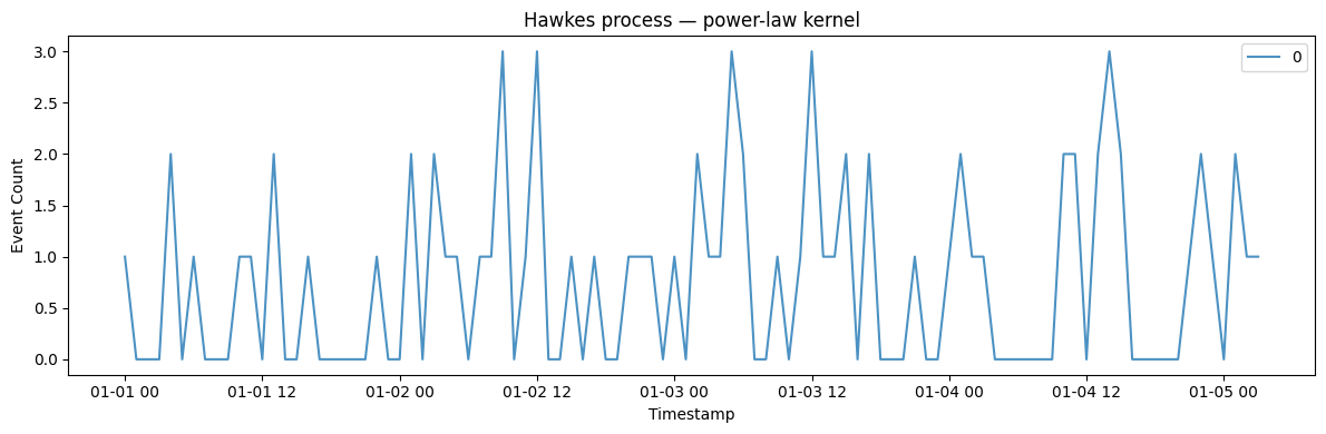
 ## 5. Power-law kernel
Use a power-law decay kernel instead of the default exponential kernel
for longer memory effects.
```python theme={null}
power_law_gen = HawkesProcessGenerator(engine="polars",
**{
"min_length": 100,
"max_length": 100,
"freq": "h",
"kernel": "power_law",
"power_law_exponent": 1.5,
"baseline_intensity": 0.5,
"excitation_amplitude": 0.2,
"seed": 42,
}
)
power_law_df = power_law_gen.generate(n_series=1)
print(f"Power-law kernel total events: {power_law_df['y'].sum()}")
```
```text theme={null}
Power-law kernel total events: 76.0
```
```python theme={null}
fig, ax = plt.subplots(figsize=(12, 4))
for uid in power_law_df["unique_id"].unique().to_list():
series = power_law_df.filter(pl.col("unique_id") == uid)
ax.plot(series["ds"].to_list(), series["y"].to_list(), label=uid, alpha=0.8)
ax.set_xlabel("Timestamp")
ax.set_ylabel("Event Count")
ax.set_title("Hawkes process — power-law kernel")
ax.legend()
plt.tight_layout()
plt.show()
```
## 5. Power-law kernel
Use a power-law decay kernel instead of the default exponential kernel
for longer memory effects.
```python theme={null}
power_law_gen = HawkesProcessGenerator(engine="polars",
**{
"min_length": 100,
"max_length": 100,
"freq": "h",
"kernel": "power_law",
"power_law_exponent": 1.5,
"baseline_intensity": 0.5,
"excitation_amplitude": 0.2,
"seed": 42,
}
)
power_law_df = power_law_gen.generate(n_series=1)
print(f"Power-law kernel total events: {power_law_df['y'].sum()}")
```
```text theme={null}
Power-law kernel total events: 76.0
```
```python theme={null}
fig, ax = plt.subplots(figsize=(12, 4))
for uid in power_law_df["unique_id"].unique().to_list():
series = power_law_df.filter(pl.col("unique_id") == uid)
ax.plot(series["ds"].to_list(), series["y"].to_list(), label=uid, alpha=0.8)
ax.set_xlabel("Timestamp")
ax.set_ylabel("Event Count")
ax.set_title("Hawkes process — power-law kernel")
ax.legend()
plt.tight_layout()
plt.show()
```
 > **Related generators**
>
> * [Poisson process](poisson_process) — the no-excitation baseline.
> * [Jump diffusion](jump_diffusion) — continuous dynamics with
> discrete shocks.
>
> Excitation and decay parameters are in the [generator
> reference](https://github.com/Nixtla/synforecast/blob/main/GENERATORS.md).
> **Related generators**
>
> * [Poisson process](poisson_process) — the no-excitation baseline.
> * [Jump diffusion](jump_diffusion) — continuous dynamics with
> discrete shocks.
>
> Excitation and decay parameters are in the [generator
> reference](https://github.com/Nixtla/synforecast/blob/main/GENERATORS.md).