> ## Documentation Index
> Fetch the complete documentation index at: https://nixtlaverse.nixtla.io/llms.txt
> Use this file to discover all available pages before exploring further.
# Probabilistic Forecasting | StatsForecast
> In this example, we’ll implement prediction intervals
> **Prerequisites**
>
> This tutorial assumes basic familiarity with StatsForecast. For a
> minimal example visit the [Quick
> Start](../getting-started/getting_started_short.html)
## Introduction
When we generate a forecast, we usually produce a single value known as
the point forecast. This value, however, doesn’t tell us anything about
the uncertainty associated with the forecast. To have a measure of this
uncertainty, we need **prediction intervals**.
A prediction interval is a range of values that the forecast can take
with a given probability. Hence, a 95% prediction interval should
contain a range of values that include the actual future value with
probability 95%. Probabilistic forecasting aims to generate the full
forecast distribution. Point forecasting, on the other hand, usually
returns the mean or the median or said distribution. However, in
real-world scenarios, it is better to forecast not only the most
probable future outcome, but many alternative outcomes as well.
[StatsForecast](../../index.html) has many models that can generate
point forecasts. It also has probabilistic models than generate the same
point forecasts and their prediction intervals. These models are
stochastic data generating processes that can produce entire forecast
distributions. By the end of this tutorial, you’ll have a good
understanding of the probabilistic models available in StatsForecast and
will be able to use them to generate point forecasts and prediction
intervals. Furthermore, you’ll also learn how to generate plots with the
historical data, the point forecasts, and the prediction intervals.
> **Important**
>
> Although the terms are often confused, prediction intervals are not
> the same as [confidence
> intervals](https://robjhyndman.com/hyndsight/intervals/).
> **Warning**
>
> In practice, most prediction intervals are too narrow since models do
> not account for all sources of uncertainty. A discussion about this
> can be found [here](https://robjhyndman.com/hyndsight/narrow-pi/).
**Outline:**
1. Install libraries
2. Load and explore the data
3. Train models
4. Plot prediction intervals
> **Tip**
>
> You can use Colab to run this Notebook interactively
>
>
>  >
## Install libraries
We assume that you have StatsForecast already installed. If not, check
this guide for instructions on [how to install
StatsForecast](../getting-started/installation.html)
Install the necessary packages using `pip install statsforecast`
```python theme={null}
%pip install -U statsforecast
```
## Load and explore the data
For this example, we’ll use the hourly dataset from the [M4
Competition](https://www.sciencedirect.com/science/article/pii/S0169207019301128).
We first need to download the data from a URL and then load it as a
`pandas` dataframe. Notice that we’ll load the train and the test data
separately. We’ll also rename the `y` column of the test data as
`y_test`.
```python theme={null}
import pandas as pd
```
```python theme={null}
train = pd.read_csv('https://auto-arima-results.s3.amazonaws.com/M4-Hourly.csv')
test = pd.read_csv('https://auto-arima-results.s3.amazonaws.com/M4-Hourly-test.csv').rename(columns={'y': 'y_test'})
```
```python theme={null}
train.head()
```
| | unique\_id | ds | y |
| - | ---------- | -- | ----- |
| 0 | H1 | 1 | 605.0 |
| 1 | H1 | 2 | 586.0 |
| 2 | H1 | 3 | 586.0 |
| 3 | H1 | 4 | 559.0 |
| 4 | H1 | 5 | 511.0 |
```python theme={null}
test.head()
```
| | unique\_id | ds | y\_test |
| - | ---------- | --- | ------- |
| 0 | H1 | 701 | 619.0 |
| 1 | H1 | 702 | 565.0 |
| 2 | H1 | 703 | 532.0 |
| 3 | H1 | 704 | 495.0 |
| 4 | H1 | 705 | 481.0 |
Since the goal of this notebook is to generate prediction intervals,
we’ll only use the first 8 series of the dataset to reduce the total
computational time.
```python theme={null}
n_series = 8
uids = train['unique_id'].unique()[:n_series] # select first n_series of the dataset
train = train.query('unique_id in @uids')
test = test.query('unique_id in @uids')
```
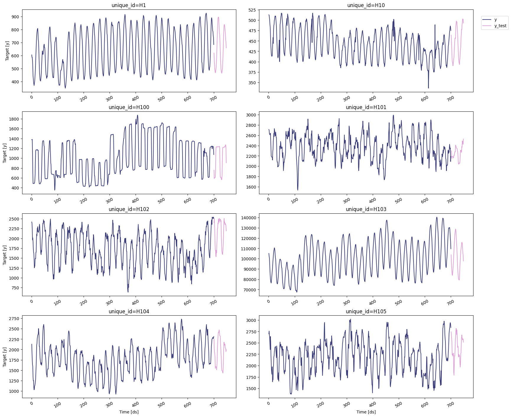
We can plot these series using the `statsforecast.plot` method from the
[StatsForecast](../../src/core/core.html#statsforecast) class. This
method has multiple parameters, and the required ones to generate the
plots in this notebook are explained below.
* `df`: A `pandas` dataframe with columns \[`unique_id`, `ds`, `y`].
* `forecasts_df`: A `pandas` dataframe with columns \[`unique_id`,
`ds`] and models.
* `plot_random`: bool = `True`. Plots the time series randomly.
* `models`: List\[str]. A list with the models we want to plot.
* `level`: List\[float]. A list with the prediction intervals we want
to plot.
* `engine`: str = `plotly`. It can also be `matplotlib`. `plotly`
generates interactive plots, while `matplotlib` generates static
plots.
```python theme={null}
from statsforecast import StatsForecast
```
```python theme={null}
StatsForecast.plot(train, test, plot_random=False)
```
>
## Install libraries
We assume that you have StatsForecast already installed. If not, check
this guide for instructions on [how to install
StatsForecast](../getting-started/installation.html)
Install the necessary packages using `pip install statsforecast`
```python theme={null}
%pip install -U statsforecast
```
## Load and explore the data
For this example, we’ll use the hourly dataset from the [M4
Competition](https://www.sciencedirect.com/science/article/pii/S0169207019301128).
We first need to download the data from a URL and then load it as a
`pandas` dataframe. Notice that we’ll load the train and the test data
separately. We’ll also rename the `y` column of the test data as
`y_test`.
```python theme={null}
import pandas as pd
```
```python theme={null}
train = pd.read_csv('https://auto-arima-results.s3.amazonaws.com/M4-Hourly.csv')
test = pd.read_csv('https://auto-arima-results.s3.amazonaws.com/M4-Hourly-test.csv').rename(columns={'y': 'y_test'})
```
```python theme={null}
train.head()
```
| | unique\_id | ds | y |
| - | ---------- | -- | ----- |
| 0 | H1 | 1 | 605.0 |
| 1 | H1 | 2 | 586.0 |
| 2 | H1 | 3 | 586.0 |
| 3 | H1 | 4 | 559.0 |
| 4 | H1 | 5 | 511.0 |
```python theme={null}
test.head()
```
| | unique\_id | ds | y\_test |
| - | ---------- | --- | ------- |
| 0 | H1 | 701 | 619.0 |
| 1 | H1 | 702 | 565.0 |
| 2 | H1 | 703 | 532.0 |
| 3 | H1 | 704 | 495.0 |
| 4 | H1 | 705 | 481.0 |
Since the goal of this notebook is to generate prediction intervals,
we’ll only use the first 8 series of the dataset to reduce the total
computational time.
```python theme={null}
n_series = 8
uids = train['unique_id'].unique()[:n_series] # select first n_series of the dataset
train = train.query('unique_id in @uids')
test = test.query('unique_id in @uids')
```
We can plot these series using the `statsforecast.plot` method from the
[StatsForecast](../../src/core/core.html#statsforecast) class. This
method has multiple parameters, and the required ones to generate the
plots in this notebook are explained below.
* `df`: A `pandas` dataframe with columns \[`unique_id`, `ds`, `y`].
* `forecasts_df`: A `pandas` dataframe with columns \[`unique_id`,
`ds`] and models.
* `plot_random`: bool = `True`. Plots the time series randomly.
* `models`: List\[str]. A list with the models we want to plot.
* `level`: List\[float]. A list with the prediction intervals we want
to plot.
* `engine`: str = `plotly`. It can also be `matplotlib`. `plotly`
generates interactive plots, while `matplotlib` generates static
plots.
```python theme={null}
from statsforecast import StatsForecast
```
```python theme={null}
StatsForecast.plot(train, test, plot_random=False)
```
 ## Train models
StatsForecast can train multiple [models](../../src/core/models.html) on
different time series efficiently. Most of these models can generate a
probabilistic forecast, which means that they can produce both point
forecasts and prediction intervals.
For this example, we’ll use
[AutoETS](../../src/core/models.html#autoets) and the following baseline
models:
* [HistoricAverage](../../src/core/models.html#historicaverage)
* [Naive](../../src/core/models.html#naive)
* [RandomWalkWithDrift](../../src/core/models.html#randomwalkwithdrift)
* [SeasonalNaive](../../src/core/models.html#seasonalnaive)
To use these models, we first need to import them from
`statsforecast.models` and then we need to instantiate them. Given that
we’re working with hourly data, we need to set `seasonal_length=24` in
the models that requiere this parameter.
```python theme={null}
from statsforecast.models import (
AutoETS,
HistoricAverage,
Naive,
RandomWalkWithDrift,
SeasonalNaive
)
```
```python theme={null}
# Create a list of models and instantiation parameters
models = [
AutoETS(season_length=24),
HistoricAverage(),
Naive(),
RandomWalkWithDrift(),
SeasonalNaive(season_length=24)
]
```
To instantiate a new StatsForecast object, we need the following
parameters:
* `df`: The dataframe with the training data.
* `models`: The list of models defined in the previous step.
* `freq`: A string indicating the frequency of the data. See [pandas’
available
frequencies](https://pandas.pydata.org/pandas-docs/stable/user_guide/timeseries.html#offset-aliases).
* `n_jobs`: An integer that indicates the number of jobs used in
parallel processing. Use -1 to select all cores.
```python theme={null}
sf = StatsForecast(
models=models,
freq=1,
n_jobs=-1
)
```
Now we’re ready to generate the point forecasts and the prediction
intervals. To do this, we’ll use the `forecast` method, which takes two
arguments:
* `h`: An integer that represent the forecasting horizon. In this
case, we’ll forecast the next 48 hours.
* `level`: A list of floats with the confidence levels of the
prediction intervals. For example, `level=[95]` means that the range
of values should include the actual future value with probability
95%.
```python theme={null}
levels = [80, 90, 95, 99] # confidence levels of the prediction intervals
forecasts = sf.forecast(df=train, h=48, level=levels)
forecasts.head()
```
| | unique\_id | ds | AutoETS | AutoETS-lo-99 | AutoETS-lo-95 | AutoETS-lo-90 | AutoETS-lo-80 | AutoETS-hi-80 | AutoETS-hi-90 | AutoETS-hi-95 | ... | RWD-hi-99 | SeasonalNaive | SeasonalNaive-lo-80 | SeasonalNaive-lo-90 | SeasonalNaive-lo-95 | SeasonalNaive-lo-99 | SeasonalNaive-hi-80 | SeasonalNaive-hi-90 | SeasonalNaive-hi-95 | SeasonalNaive-hi-99 |
| - | ---------- | --- | ---------- | ------------- | ------------- | ------------- | ------------- | ------------- | ------------- | ------------- | --- | ---------- | ------------- | ------------------- | ------------------- | ------------------- | ------------------- | ------------------- | ------------------- | ------------------- | ------------------- |
| 0 | H1 | 701 | 631.889598 | 533.371822 | 556.926831 | 568.978861 | 582.874079 | 680.905116 | 694.800335 | 706.852365 | ... | 789.416619 | 691.0 | 613.351903 | 591.339747 | 572.247484 | 534.932739 | 768.648097 | 790.660253 | 809.752516 | 847.067261 |
| 1 | H1 | 702 | 559.750830 | 460.738592 | 484.411824 | 496.524343 | 510.489302 | 609.012359 | 622.977317 | 635.089836 | ... | 833.254152 | 618.0 | 540.351903 | 518.339747 | 499.247484 | 461.932739 | 695.648097 | 717.660253 | 736.752516 | 774.067261 |
| 2 | H1 | 703 | 519.235476 | 419.731233 | 443.522100 | 455.694808 | 469.729161 | 568.741792 | 582.776145 | 594.948853 | ... | 866.990616 | 563.0 | 485.351903 | 463.339747 | 444.247484 | 406.932739 | 640.648097 | 662.660253 | 681.752516 | 719.067261 |
| 3 | H1 | 704 | 486.973364 | 386.979536 | 410.887460 | 423.120060 | 437.223465 | 536.723263 | 550.826668 | 563.059268 | ... | 895.510095 | 529.0 | 451.351903 | 429.339747 | 410.247484 | 372.932739 | 606.648097 | 628.660253 | 647.752516 | 685.067261 |
| 4 | H1 | 705 | 464.697366 | 364.216339 | 388.240749 | 400.532950 | 414.705071 | 514.689661 | 528.861782 | 541.153983 | ... | 920.702904 | 504.0 | 426.351903 | 404.339747 | 385.247484 | 347.932739 | 581.648097 | 603.660253 | 622.752516 | 660.067261 |
We’ll now merge the forecasts and their prediction intervals with the
test set. This will allow us generate the plots of each probabilistic
model.
```python theme={null}
test = test.merge(forecasts, how='left', on=['unique_id', 'ds'])
```
## Plot prediction intervals
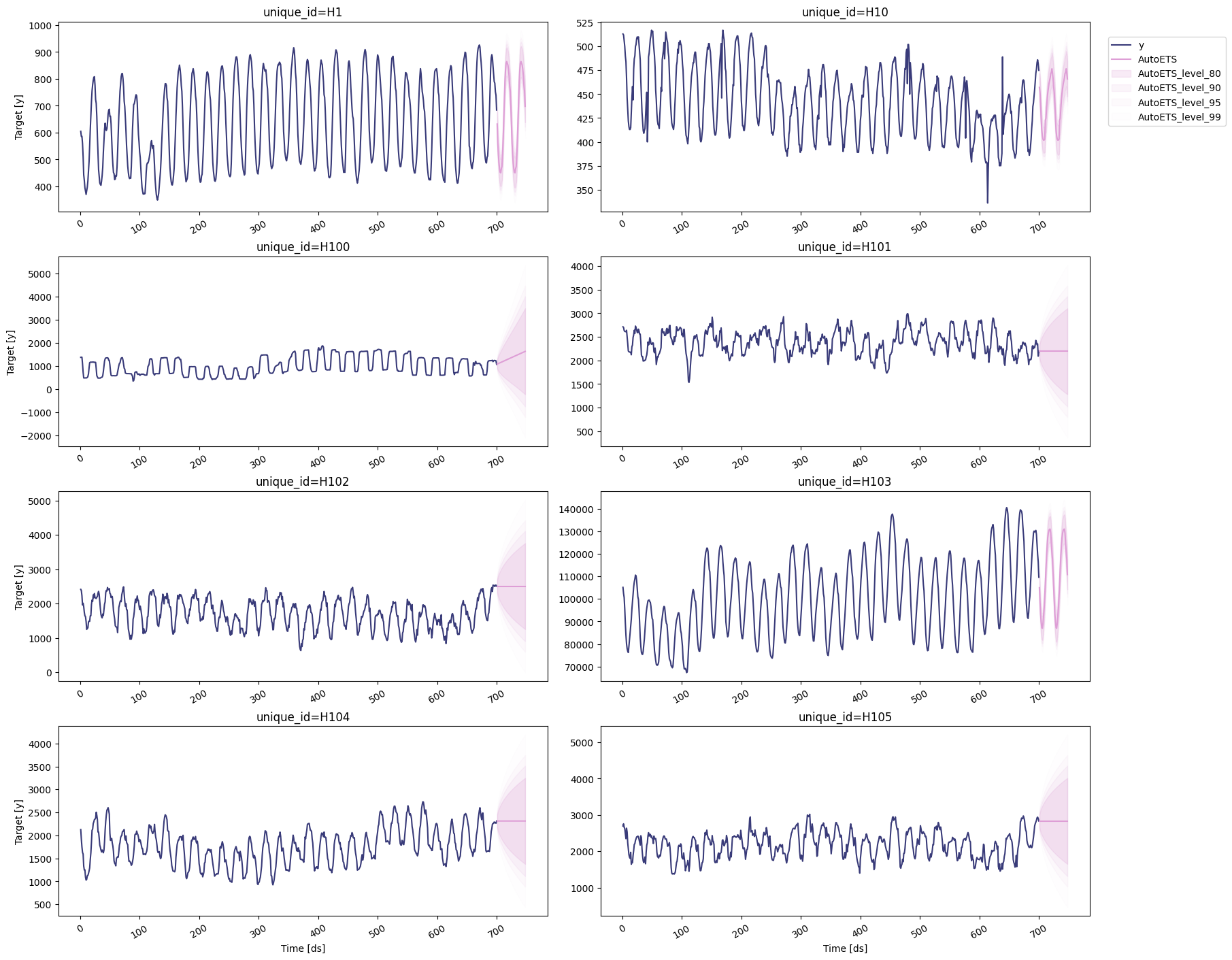
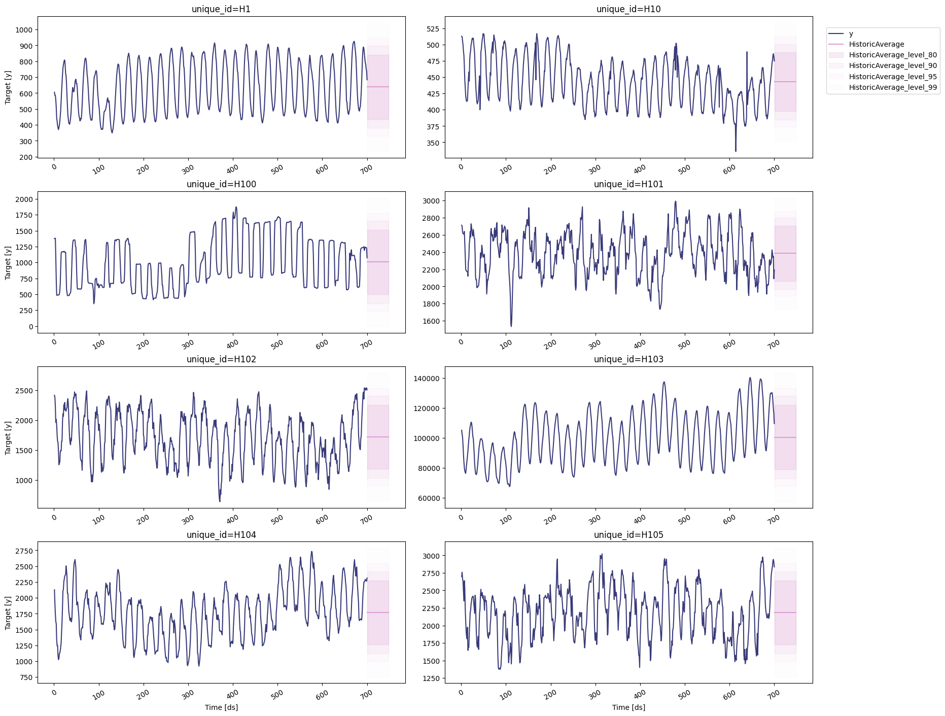
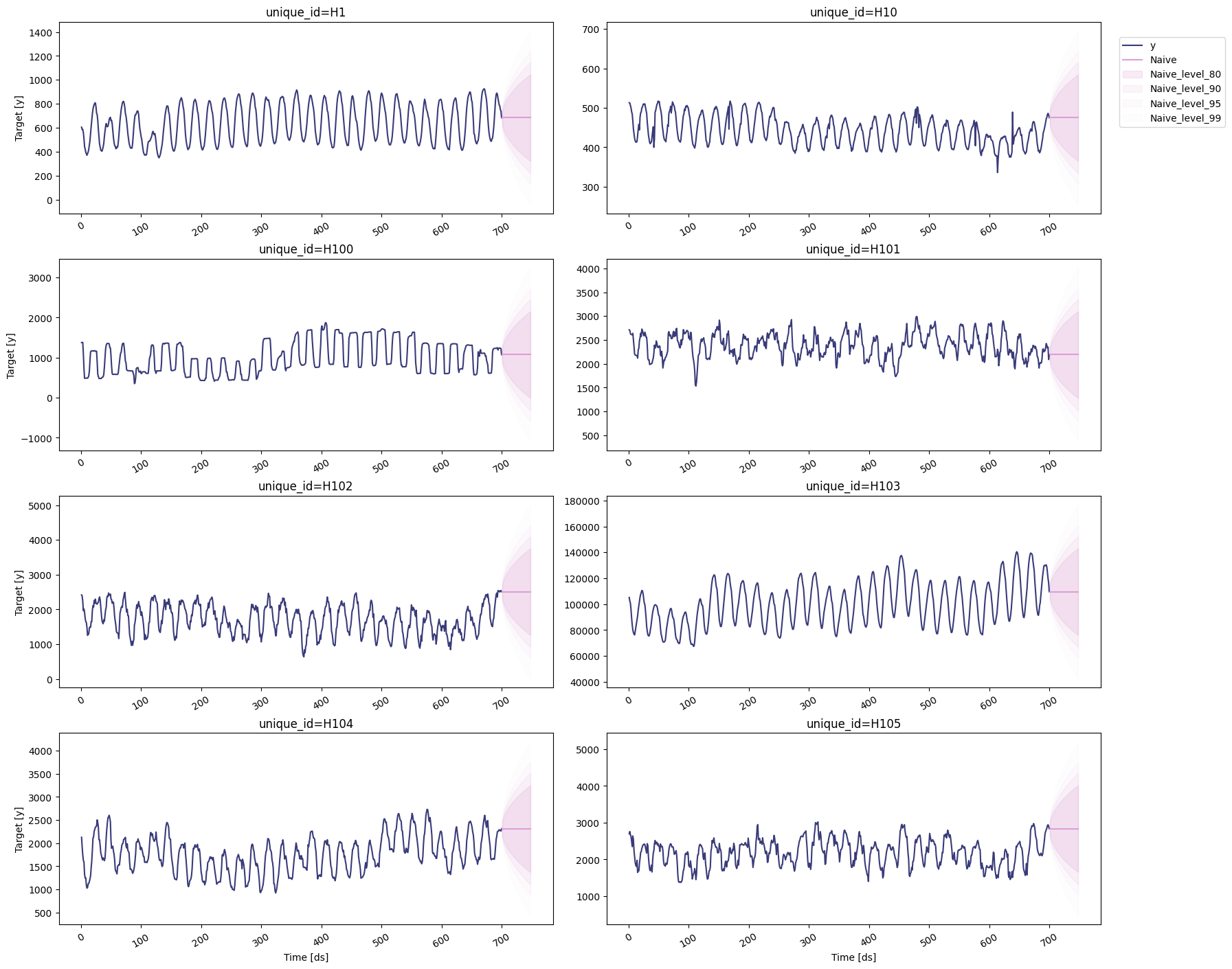
To plot the point and the prediction intervals, we’ll use the
`statsforecast.plot` method again. Notice that now we also need to
specify the model and the levels that we want to plot.
### AutoETS
```python theme={null}
sf.plot(train, test, plot_random=False, models=['AutoETS'], level=levels)
```
## Train models
StatsForecast can train multiple [models](../../src/core/models.html) on
different time series efficiently. Most of these models can generate a
probabilistic forecast, which means that they can produce both point
forecasts and prediction intervals.
For this example, we’ll use
[AutoETS](../../src/core/models.html#autoets) and the following baseline
models:
* [HistoricAverage](../../src/core/models.html#historicaverage)
* [Naive](../../src/core/models.html#naive)
* [RandomWalkWithDrift](../../src/core/models.html#randomwalkwithdrift)
* [SeasonalNaive](../../src/core/models.html#seasonalnaive)
To use these models, we first need to import them from
`statsforecast.models` and then we need to instantiate them. Given that
we’re working with hourly data, we need to set `seasonal_length=24` in
the models that requiere this parameter.
```python theme={null}
from statsforecast.models import (
AutoETS,
HistoricAverage,
Naive,
RandomWalkWithDrift,
SeasonalNaive
)
```
```python theme={null}
# Create a list of models and instantiation parameters
models = [
AutoETS(season_length=24),
HistoricAverage(),
Naive(),
RandomWalkWithDrift(),
SeasonalNaive(season_length=24)
]
```
To instantiate a new StatsForecast object, we need the following
parameters:
* `df`: The dataframe with the training data.
* `models`: The list of models defined in the previous step.
* `freq`: A string indicating the frequency of the data. See [pandas’
available
frequencies](https://pandas.pydata.org/pandas-docs/stable/user_guide/timeseries.html#offset-aliases).
* `n_jobs`: An integer that indicates the number of jobs used in
parallel processing. Use -1 to select all cores.
```python theme={null}
sf = StatsForecast(
models=models,
freq=1,
n_jobs=-1
)
```
Now we’re ready to generate the point forecasts and the prediction
intervals. To do this, we’ll use the `forecast` method, which takes two
arguments:
* `h`: An integer that represent the forecasting horizon. In this
case, we’ll forecast the next 48 hours.
* `level`: A list of floats with the confidence levels of the
prediction intervals. For example, `level=[95]` means that the range
of values should include the actual future value with probability
95%.
```python theme={null}
levels = [80, 90, 95, 99] # confidence levels of the prediction intervals
forecasts = sf.forecast(df=train, h=48, level=levels)
forecasts.head()
```
| | unique\_id | ds | AutoETS | AutoETS-lo-99 | AutoETS-lo-95 | AutoETS-lo-90 | AutoETS-lo-80 | AutoETS-hi-80 | AutoETS-hi-90 | AutoETS-hi-95 | ... | RWD-hi-99 | SeasonalNaive | SeasonalNaive-lo-80 | SeasonalNaive-lo-90 | SeasonalNaive-lo-95 | SeasonalNaive-lo-99 | SeasonalNaive-hi-80 | SeasonalNaive-hi-90 | SeasonalNaive-hi-95 | SeasonalNaive-hi-99 |
| - | ---------- | --- | ---------- | ------------- | ------------- | ------------- | ------------- | ------------- | ------------- | ------------- | --- | ---------- | ------------- | ------------------- | ------------------- | ------------------- | ------------------- | ------------------- | ------------------- | ------------------- | ------------------- |
| 0 | H1 | 701 | 631.889598 | 533.371822 | 556.926831 | 568.978861 | 582.874079 | 680.905116 | 694.800335 | 706.852365 | ... | 789.416619 | 691.0 | 613.351903 | 591.339747 | 572.247484 | 534.932739 | 768.648097 | 790.660253 | 809.752516 | 847.067261 |
| 1 | H1 | 702 | 559.750830 | 460.738592 | 484.411824 | 496.524343 | 510.489302 | 609.012359 | 622.977317 | 635.089836 | ... | 833.254152 | 618.0 | 540.351903 | 518.339747 | 499.247484 | 461.932739 | 695.648097 | 717.660253 | 736.752516 | 774.067261 |
| 2 | H1 | 703 | 519.235476 | 419.731233 | 443.522100 | 455.694808 | 469.729161 | 568.741792 | 582.776145 | 594.948853 | ... | 866.990616 | 563.0 | 485.351903 | 463.339747 | 444.247484 | 406.932739 | 640.648097 | 662.660253 | 681.752516 | 719.067261 |
| 3 | H1 | 704 | 486.973364 | 386.979536 | 410.887460 | 423.120060 | 437.223465 | 536.723263 | 550.826668 | 563.059268 | ... | 895.510095 | 529.0 | 451.351903 | 429.339747 | 410.247484 | 372.932739 | 606.648097 | 628.660253 | 647.752516 | 685.067261 |
| 4 | H1 | 705 | 464.697366 | 364.216339 | 388.240749 | 400.532950 | 414.705071 | 514.689661 | 528.861782 | 541.153983 | ... | 920.702904 | 504.0 | 426.351903 | 404.339747 | 385.247484 | 347.932739 | 581.648097 | 603.660253 | 622.752516 | 660.067261 |
We’ll now merge the forecasts and their prediction intervals with the
test set. This will allow us generate the plots of each probabilistic
model.
```python theme={null}
test = test.merge(forecasts, how='left', on=['unique_id', 'ds'])
```
## Plot prediction intervals
To plot the point and the prediction intervals, we’ll use the
`statsforecast.plot` method again. Notice that now we also need to
specify the model and the levels that we want to plot.
### AutoETS
```python theme={null}
sf.plot(train, test, plot_random=False, models=['AutoETS'], level=levels)
```
 ### Historic Average
```python theme={null}
sf.plot(train, test, plot_random=False, models=['HistoricAverage'], level=levels)
```
### Historic Average
```python theme={null}
sf.plot(train, test, plot_random=False, models=['HistoricAverage'], level=levels)
```
 ### Naive
```python theme={null}
sf.plot(train, test, plot_random=False, models=['Naive'], level=levels)
```
### Naive
```python theme={null}
sf.plot(train, test, plot_random=False, models=['Naive'], level=levels)
```
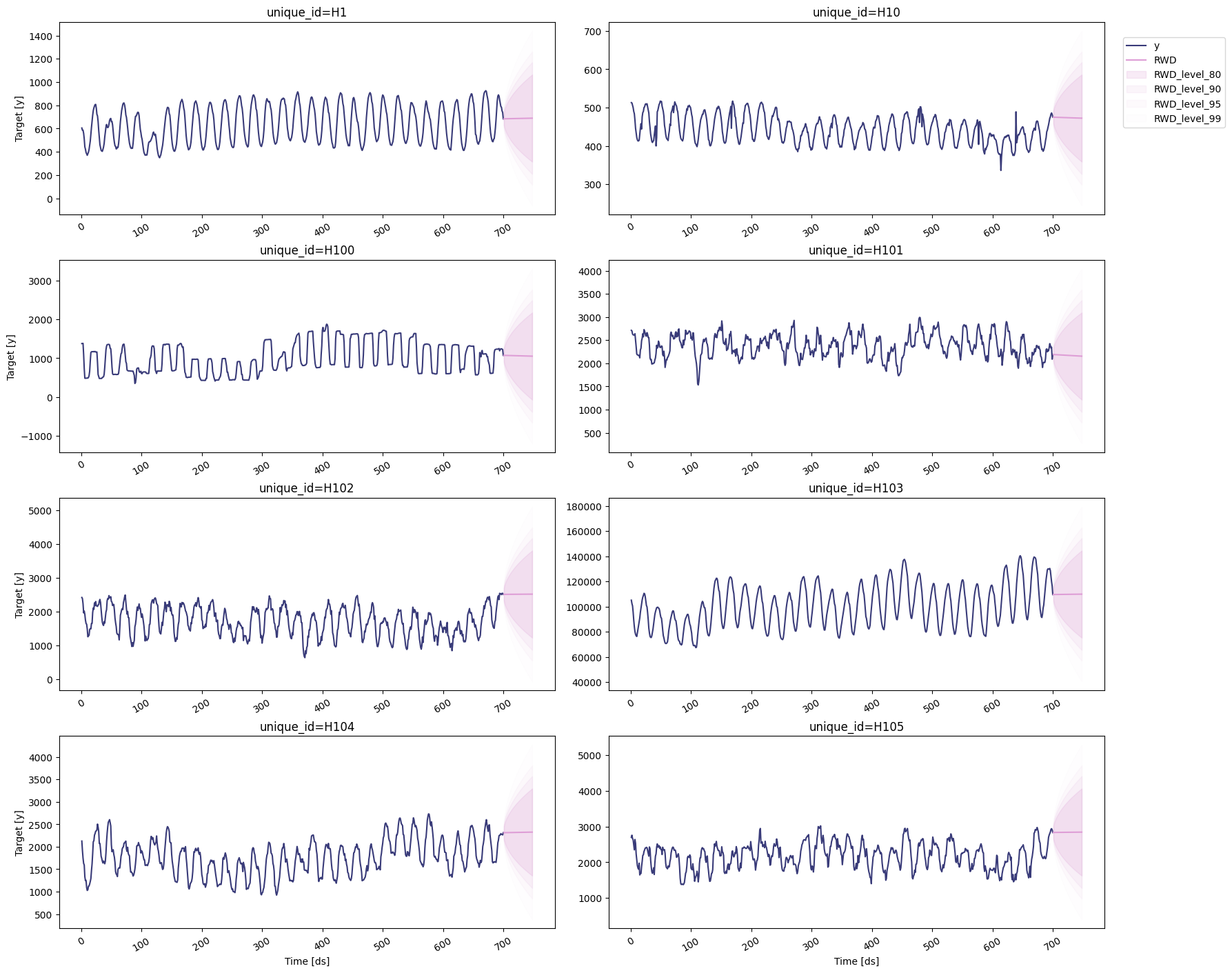
 ### Random Walk with Drift
```python theme={null}
sf.plot(train, test, plot_random=False, models=['RWD'], level=levels)
```
### Random Walk with Drift
```python theme={null}
sf.plot(train, test, plot_random=False, models=['RWD'], level=levels)
```
 ### Seasonal Naive
```python theme={null}
sf.plot(train, test, plot_random=False, models=['SeasonalNaive'], level=levels)
```
### Seasonal Naive
```python theme={null}
sf.plot(train, test, plot_random=False, models=['SeasonalNaive'], level=levels)
```
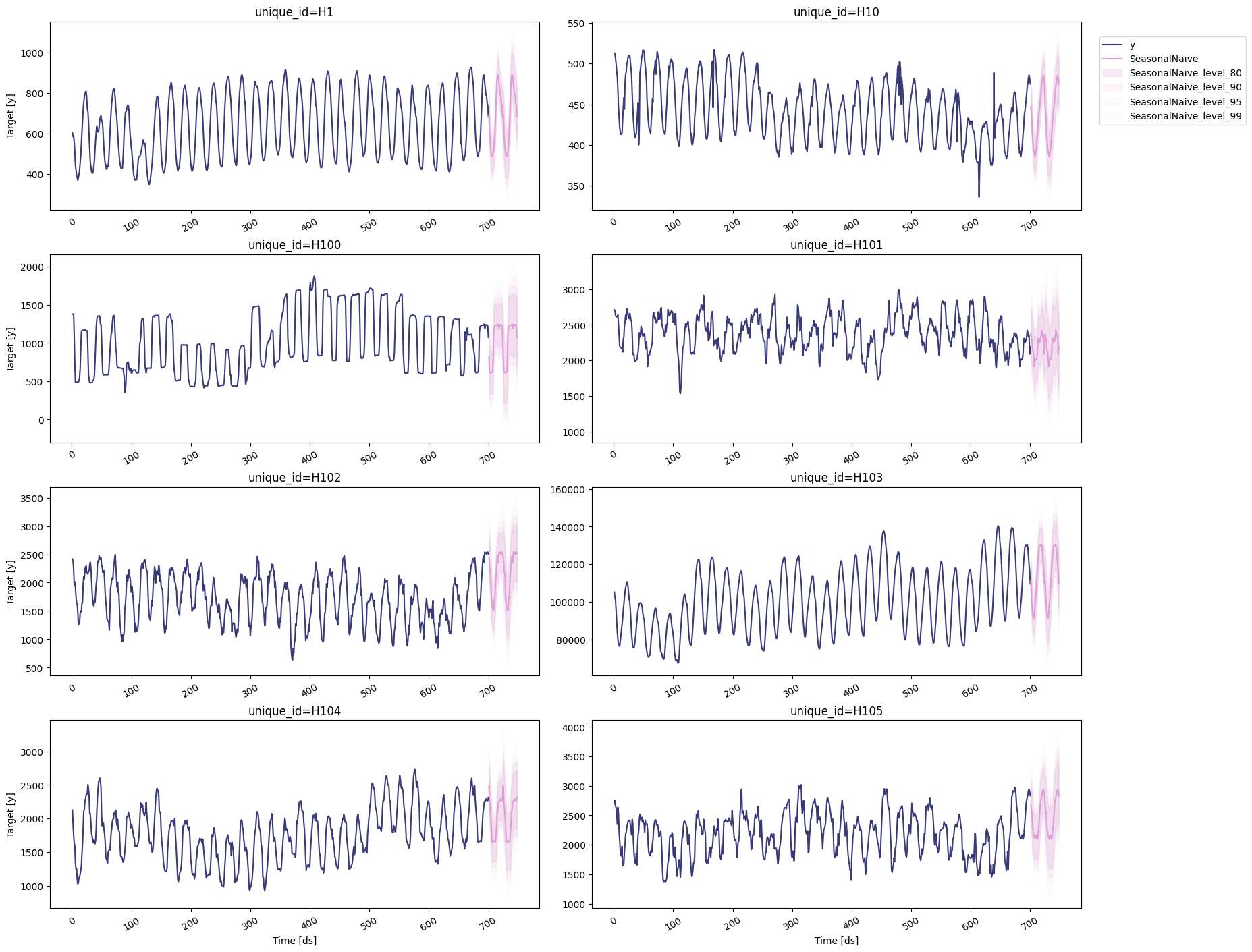 From these plots, we can conclude that the uncertainty around each
forecast varies according to the model that is being used. For the same
time series, one model can predict a wider range of possible future
values than others.
## References
[Rob J. Hyndman and George Athanasopoulos (2018). “Forecasting
principles and practice, The Statistical Forecasting
Perspective”](https://otexts.com/fpp3/perspective.html).
From these plots, we can conclude that the uncertainty around each
forecast varies according to the model that is being used. For the same
time series, one model can predict a wider range of possible future
values than others.
## References
[Rob J. Hyndman and George Athanasopoulos (2018). “Forecasting
principles and practice, The Statistical Forecasting
Perspective”](https://otexts.com/fpp3/perspective.html).