> ## Documentation Index
> Fetch the complete documentation index at: https://nixtlaverse.nixtla.io/llms.txt
> Use this file to discover all available pages before exploring further.
# Statistical, Machine Learning and Neural Forecasting methods | StatsForecast
> In this notebook, you will make forecasts for the M5 dataset choosing
> the best model for each time series using cross validation.
Statistical, Machine Learning, and Neural Forecasting Methods In this
tutorial, we will explore the process of forecasting on the M5 dataset
by utilizing the most suitable model for each time series. We’ll
accomplish this through an essential technique known as
cross-validation. This approach helps us in estimating the predictive
performance of our models, and in selecting the model that yields the
best performance for each time series.
The M5 dataset comprises of hierarchical sales data, spanning five
years, from Walmart. The aim is to forecast daily sales for the next 28
days. The dataset is broken down into the 50 states of America, with 10
stores in each state.
In the realm of time series forecasting and analysis, one of the more
complex tasks is identifying the model that is optimally suited for a
specific group of series. Quite often, this selection process leans
heavily on intuition, which may not necessarily align with the empirical
reality of our dataset.
In this tutorial, we aim to provide a more structured, data-driven
approach to model selection for different groups of series within the M5
benchmark dataset. This dataset, well-known in the field of forecasting,
allows us to showcase the versatility and power of our methodology.
We will train an assortment of models from various forecasting
paradigms:
*[StatsForecast](https://github.com/Nixtla/statsforecast)*
* Baseline models: These models are simple yet often highly effective
for providing an initial perspective on the forecasting problem. We
will use `SeasonalNaive` and `HistoricAverage` models for this
category.
* Intermittent models: For series with sporadic, non-continuous
demand, we will utilize models like `CrostonOptimized`, `IMAPA`, and
`ADIDA`. These models are particularly suited for handling
zero-inflated series.
* State Space Models: These are statistical models that use
mathematical descriptions of a system to make predictions. The
`AutoETS` model from the statsforecast library falls under this
category.
*[MLForecast](https://github.com/Nixtla/mlforecast)*
Machine Learning: Leveraging ML models like `LightGBM`, `XGBoost`, and
`LinearRegression` can be advantageous due to their capacity to uncover
intricate patterns in data. We’ll use the MLForecast library for this
purpose.
*[NeuralForecast](https://github.com/Nixtla/neuralforecast)*
Deep Learning: DL models, such as Transformers (`AutoTFT`) and Neural
Networks (`AutoNHITS`), allow us to handle complex non-linear
dependencies in time series data. We’ll utilize the NeuralForecast
library for these models.
Using the Nixtla suite of libraries, we’ll be able to drive our model
selection process with data, ensuring we utilize the most suitable
models for specific groups of series in our dataset.
Outline:
* Reading Data: In this initial step, we load our dataset into memory,
making it available for our subsequent analysis and forecasting. It
is important to understand the structure and nuances of the dataset
at this stage.
* Forecasting Using Statistical and Deep Learning Methods: We apply a
wide range of forecasting methods from basic statistical techniques
to advanced deep learning models. The aim is to generate predictions
for the next 28 days based on our dataset.
* Model Performance Evaluation on Different Windows: We assess the
performance of our models on distinct windows.
* Selecting the Best Model for a Group of Series: Using the
performance evaluation, we identify the optimal model for each group
of series. This step ensures that the chosen model is tailored to
the unique characteristics of each group.
* Filtering the Best Possible Forecast: Finally, we filter the
forecasts generated by our chosen models to obtain the most
promising predictions. This is our final output and represents the
best possible forecast for each series according to our models.
> **Warning**
>
> This tutorial was originally executed using a `c5d.24xlarge` EC2
> instance.
## Installing Libraries
```python theme={null}
%%capture
!pip install statsforecast mlforecast neuralforecast datasetforecast s3fs pyarrow
```
## Download and prepare data
The example uses the [M5
dataset](https://github.com/Mcompetitions/M5-methods/blob/master/M5-Competitors-Guide.pdf).
It consists of `30,490` bottom time series.
```python theme={null}
import pandas as pd
```
```python theme={null}
# Load the training target dataset from the provided URL
Y_df = pd.read_parquet('https://m5-benchmarks.s3.amazonaws.com/data/train/target.parquet')
# Rename columns to match the Nixtlaverse's expectations
# The 'item_id' becomes 'unique_id' representing the unique identifier of the time series
# The 'timestamp' becomes 'ds' representing the time stamp of the data points
# The 'demand' becomes 'y' representing the target variable we want to forecast
Y_df = Y_df.rename(columns={
'item_id': 'unique_id',
'timestamp': 'ds',
'demand': 'y'
})
# Convert the 'ds' column to datetime format to ensure proper handling of date-related operations in subsequent steps
Y_df['ds'] = pd.to_datetime(Y_df['ds'])
```
For simplicity sake we will keep just one category
```python theme={null}
Y_df = Y_df.query('unique_id.str.startswith("FOODS_3")').reset_index(drop=True)
Y_df['unique_id'] = Y_df['unique_id'].astype(str)
```
# Basic Plotting
Plot some series using the plot method from the `StatsForecast` class.
This method prints 8 random series from the dataset and is useful for
basic [EDA](../../src/core/core.html#plot).
```python theme={null}
from statsforecast import StatsForecast
```
```python theme={null}
# Feature: plot random series for EDA
StatsForecast.plot(Y_df)
```
```python theme={null}
# Feature: plot groups of series for EDA
StatsForecast.plot(Y_df, unique_ids=["FOODS_3_432_TX_2"])
```
```python theme={null}
# Feature: plot groups of series for EDA
StatsForecast.plot(Y_df, unique_ids=["FOODS_3_432_TX_2"], engine ='matplotlib')
```
# Create forecasts with Stats, Ml and Neural methods.
## StatsForecast
`StatsForecast` is a comprehensive library providing a suite of popular
univariate time series forecasting models, all designed with a focus on
high performance and scalability.
Here’s what makes StatsForecast a powerful tool for time series
forecasting:
* **Collection of Local Models**: StatsForecast provides a diverse
collection of local models that can be applied to each time series
individually, allowing us to capture unique patterns within each
series.
* **Simplicity**: With StatsForecast, training, forecasting, and
backtesting multiple models become a straightforward process,
requiring only a few lines of code. This simplicity makes it a
convenient tool for both beginners and experienced practitioners.
* **Optimized for Speed**: The implementation of the models in
StatsForecast is optimized for speed, ensuring that large-scale
computations are performed efficiently, thereby reducing the overall
time for model training and prediction.
* **Horizontal Scalability**: One of the distinguishing features of
StatsForecast is its ability to scale horizontally. It is compatible
with distributed computing frameworks such as Spark, Dask, and Ray.
This feature allows it to handle large datasets by distributing the
computations across multiple nodes in a cluster, making it a go-to
solution for large-scale time series forecasting tasks.
`StatsForecast` receives a list of models to fit each time series. Since
we are dealing with Daily data, it would be beneficial to use 7 as
seasonality.
```python theme={null}
# Import necessary models from the statsforecast library
from statsforecast.models import (
# SeasonalNaive: A model that uses the previous season's data as the forecast
SeasonalNaive,
# Naive: A simple model that uses the last observed value as the forecast
Naive,
# HistoricAverage: This model uses the average of all historical data as the forecast
HistoricAverage,
# CrostonOptimized: A model specifically designed for intermittent demand forecasting
CrostonOptimized,
# ADIDA: Adaptive combination of Intermittent Demand Approaches, a model designed for intermittent demand
ADIDA,
# IMAPA: Intermittent Multiplicative AutoRegressive Average, a model for intermittent series that incorporates autocorrelation
IMAPA,
# AutoETS: Automated Exponential Smoothing model that automatically selects the best Exponential Smoothing model based on AIC
AutoETS
)
```
We fit the models by instantiating a new StatsForecast object with the
following parameters:
* `models`: a list of models. Select the models you want from models
and import them.
* `freq`: a string indicating the frequency of the data. (See panda’s
available frequencies.)
* `n_jobs`: int, number of jobs used in the parallel processing, use
-1 for all cores.
* `fallback_model`: a model to be used if a model fails. Any settings
are passed into the constructor. Then you call its fit method and
pass in the historical data frame.
```python theme={null}
horizon = 28
models = [
SeasonalNaive(season_length=7),
Naive(),
HistoricAverage(),
CrostonOptimized(),
ADIDA(),
IMAPA(),
AutoETS(season_length=7)
]
```
```python theme={null}
# Instantiate the StatsForecast class
sf = StatsForecast(
models=models, # A list of models to be used for forecasting
freq='D', # The frequency of the time series data (in this case, 'D' stands for daily frequency)
n_jobs=-1, # The number of CPU cores to use for parallel execution (-1 means use all available cores)
)
```
The forecast method takes two arguments: forecasts next h (horizon) and
level.
* `h` (int): represents the forecast h steps into the future. In this
case, 12 months ahead.
* `level` (list of floats): this optional parameter is used for
probabilistic forecasting. Set the level (or confidence percentile)
of your prediction interval. For example, level=\[90] means that
the model expects the real value to be inside that interval 90% of
the times.
The forecast object here is a new data frame that includes a column with
the name of the model and the y hat values, as well as columns for the
uncertainty intervals.
This block of code times how long it takes to run the forecasting
function of the StatsForecast class, which predicts the next 28 days
(h=28). The level is set to \[90], meaning it will compute the 90%
prediction interval. The time is calculated in minutes and printed out
at the end.
```python theme={null}
from time import time
# Get the current time before forecasting starts, this will be used to measure the execution time
init = time()
# Call the forecast method of the StatsForecast instance to predict the next 28 days (h=28)
# Level is set to [90], which means that it will compute the 90% prediction interval
fcst_df = sf.forecast(df=Y_df, h=28, level=[90])
# Get the current time after the forecasting ends
end = time()
# Calculate and print the total time taken for the forecasting in minutes
print(f'Forecast Minutes: {(end - init) / 60}')
```
```text theme={null}
Forecast Minutes: 2.270755163828532
```
```python theme={null}
fcst_df.head()
```
| | ds | SeasonalNaive | SeasonalNaive-lo-90 | SeasonalNaive-hi-90 | Naive | Naive-lo-90 | Naive-hi-90 | HistoricAverage | HistoricAverage-lo-90 | HistoricAverage-hi-90 | CrostonOptimized | ADIDA | IMAPA | AutoETS | AutoETS-lo-90 | AutoETS-hi-90 |
| -------------------- | ---------- | ------------- | ------------------- | ------------------- | ----- | ----------- | ----------- | --------------- | --------------------- | --------------------- | ---------------- | -------- | -------- | -------- | ------------- | ------------- |
| unique\_id | | | | | | | | | | | | | | | | |
| FOODS\_3\_001\_CA\_1 | 2016-05-23 | 1.0 | -2.847174 | 4.847174 | 2.0 | 0.098363 | 3.901637 | 0.448738 | -1.009579 | 1.907055 | 0.345192 | 0.345477 | 0.347249 | 0.381414 | -1.028122 | 1.790950 |
| FOODS\_3\_001\_CA\_1 | 2016-05-24 | 0.0 | -3.847174 | 3.847174 | 2.0 | -0.689321 | 4.689321 | 0.448738 | -1.009579 | 1.907055 | 0.345192 | 0.345477 | 0.347249 | 0.286933 | -1.124136 | 1.698003 |
| FOODS\_3\_001\_CA\_1 | 2016-05-25 | 0.0 | -3.847174 | 3.847174 | 2.0 | -1.293732 | 5.293732 | 0.448738 | -1.009579 | 1.907055 | 0.345192 | 0.345477 | 0.347249 | 0.334987 | -1.077614 | 1.747588 |
| FOODS\_3\_001\_CA\_1 | 2016-05-26 | 1.0 | -2.847174 | 4.847174 | 2.0 | -1.803274 | 5.803274 | 0.448738 | -1.009579 | 1.907055 | 0.345192 | 0.345477 | 0.347249 | 0.186851 | -1.227280 | 1.600982 |
| FOODS\_3\_001\_CA\_1 | 2016-05-27 | 0.0 | -3.847174 | 3.847174 | 2.0 | -2.252190 | 6.252190 | 0.448738 | -1.009579 | 1.907055 | 0.345192 | 0.345477 | 0.347249 | 0.308112 | -1.107548 | 1.723771 |
## MLForecast
`MLForecast` is a powerful library that provides automated feature
creation for time series forecasting, facilitating the use of global
machine learning models. It is designed for high performance and
scalability.
Key features of MLForecast include:
* **Support for sklearn models**: MLForecast is compatible with models
that follow the scikit-learn API. This makes it highly flexible and
allows it to seamlessly integrate with a wide variety of machine
learning algorithms.
* **Simplicity**: With MLForecast, the tasks of training, forecasting,
and backtesting models can be accomplished in just a few lines of
code. This streamlined simplicity makes it user-friendly for
practitioners at all levels of expertise.
* **Optimized for speed:** MLForecast is engineered to execute tasks
rapidly, which is crucial when handling large datasets and complex
models.
* **Horizontal Scalability:** MLForecast is capable of horizontal
scaling using distributed computing frameworks such as Spark, Dask,
and Ray. This feature enables it to efficiently process massive
datasets by distributing the computations across multiple nodes in a
cluster, making it ideal for large-scale time series forecasting
tasks.
```python theme={null}
from mlforecast import MLForecast
from mlforecast.target_transforms import Differences
from mlforecast.utils import PredictionIntervals
from window_ops.expanding import expanding_mean
```
```python theme={null}
%%capture
!pip install lightgbm xgboost
```
```python theme={null}
# Import the necessary models from various libraries
# LGBMRegressor: A gradient boosting framework that uses tree-based learning algorithms from the LightGBM library
from lightgbm import LGBMRegressor
# XGBRegressor: A gradient boosting regressor model from the XGBoost library
from xgboost import XGBRegressor
# LinearRegression: A simple linear regression model from the scikit-learn library
from sklearn.linear_model import LinearRegression
```
To use `MLForecast` for time series forecasting, we instantiate a new
`MLForecast` object and provide it with various parameters to tailor the
modeling process to our specific needs:
* `models`: This parameter accepts a list of machine learning models
you wish to use for forecasting. You can import your preferred
models from scikit-learn, lightgbm and xgboost.
* `freq`: This is a string indicating the frequency of your data
(hourly, daily, weekly, etc.). The specific format of this string
should align with pandas’ recognized frequency strings.
* `target_transforms`: These are transformations applied to the target
variable before model training and after model prediction. This can
be useful when working with data that may benefit from
transformations, such as log-transforms for highly skewed data.
* `lags`: This parameter accepts specific lag values to be used as
regressors. Lags represent how many steps back in time you want to
look when creating features for your model. For example, if you want
to use the previous day’s data as a feature for predicting today’s
value, you would specify a lag of 1.
* `lags_transforms`: These are specific transformations for each lag.
This allows you to apply transformations to your lagged features.
* `date_features`: This parameter specifies date-related features to
be used as regressors. For instance, you might want to include the
day of the week or the month as a feature in your model.
* `num_threads`: This parameter controls the number of threads to use
for parallelizing feature creation, helping to speed up this process
when working with large datasets.
All these settings are passed to the `MLForecast` constructor. Once the
`MLForecast` object is initialized with these settings, we call its
`fit` method and pass the historical data frame as the argument. The
`fit` method trains the models on the provided historical data, readying
them for future forecasting tasks.
```python theme={null}
# Instantiate the MLForecast object
mlf = MLForecast(
models=[LGBMRegressor(), XGBRegressor(), LinearRegression()], # List of models for forecasting: LightGBM, XGBoost and Linear Regression
freq='D', # Frequency of the data - 'D' for daily frequency
lags=list(range(1, 7)), # Specific lags to use as regressors: 1 to 6 days
lag_transforms = {
1: [expanding_mean], # Apply expanding mean transformation to the lag of 1 day
},
date_features=['year', 'month', 'day', 'dayofweek', 'quarter', 'week'], # Date features to use as regressors
)
```
Just call the `fit` models to train the select models. In this case we
are generating conformal prediction intervals.
```python theme={null}
# Start the timer to calculate the time taken for fitting the models
init = time()
# Fit the MLForecast models to the data, with prediction intervals set using a window size of 28 days
mlf.fit(Y_df, prediction_intervals=PredictionIntervals(window_size=28))
# Calculate the end time after fitting the models
end = time()
# Print the time taken to fit the MLForecast models, in minutes
print(f'MLForecast Minutes: {(end - init) / 60}')
```
```text theme={null}
MLForecast Minutes: 2.2809854547182717
```
After that, just call `predict` to generate forecasts.
```python theme={null}
fcst_mlf_df = mlf.predict(28, level=[90])
```
```python theme={null}
fcst_mlf_df.head()
```
| | unique\_id | ds | LGBMRegressor | XGBRegressor | LinearRegression | LGBMRegressor-lo-90 | LGBMRegressor-hi-90 | XGBRegressor-lo-90 | XGBRegressor-hi-90 | LinearRegression-lo-90 | LinearRegression-hi-90 |
| - | -------------------- | ---------- | ------------- | ------------ | ---------------- | ------------------- | ------------------- | ------------------ | ------------------ | ---------------------- | ---------------------- |
| 0 | FOODS\_3\_001\_CA\_1 | 2016-05-23 | 0.549520 | 0.598431 | 0.359638 | -0.213915 | 1.312955 | -0.020050 | 1.216912 | 0.030000 | 0.689277 |
| 1 | FOODS\_3\_001\_CA\_1 | 2016-05-24 | 0.553196 | 0.337268 | 0.100361 | -0.251383 | 1.357775 | -0.201449 | 0.875985 | -0.216195 | 0.416917 |
| 2 | FOODS\_3\_001\_CA\_1 | 2016-05-25 | 0.599668 | 0.349604 | 0.175840 | -0.203974 | 1.403309 | -0.284416 | 0.983624 | -0.150593 | 0.502273 |
| 3 | FOODS\_3\_001\_CA\_1 | 2016-05-26 | 0.638097 | 0.322144 | 0.156460 | 0.118688 | 1.157506 | -0.085872 | 0.730160 | -0.273851 | 0.586771 |
| 4 | FOODS\_3\_001\_CA\_1 | 2016-05-27 | 0.763305 | 0.300362 | 0.328194 | -0.313091 | 1.839701 | -0.296636 | 0.897360 | -0.657089 | 1.313476 |
## NeuralForecast
`NeuralForecast` is a robust collection of neural forecasting models
that focuses on usability and performance. It includes a variety of
model architectures, from classic networks such as Multilayer
Perceptrons (MLP) and Recurrent Neural Networks (RNN) to novel
contributions like N-BEATS, N-HITS, Temporal Fusion Transformers (TFT),
and more.
Key features of `NeuralForecast` include:
* A broad collection of global models. Out of the box implementation
of MLP, LSTM, RNN, TCN, DilatedRNN, NBEATS, NHITS, ESRNN, TFT,
Informer, PatchTST and HINT.
* A simple and intuitive interface that allows training, forecasting,
and backtesting of various models in a few lines of code.
* Support for GPU acceleration to improve computational speed.
This machine doesn’t have GPU, but Google Colabs offers some for free.
Using [Colab’s GPU to train
NeuralForecast](../../../neuralforecast/docs/tutorials/intermittent_data.html).
```python theme={null}
# Read the results from Colab
fcst_nf_df = pd.read_parquet('https://m5-benchmarks.s3.amazonaws.com/data/forecast-nf.parquet')
```
```python theme={null}
fcst_nf_df.head()
```
| | unique\_id | ds | AutoNHITS | AutoNHITS-lo-90 | AutoNHITS-hi-90 | AutoTFT | AutoTFT-lo-90 | AutoTFT-hi-90 |
| - | -------------------- | ---------- | --------- | --------------- | --------------- | ------- | ------------- | ------------- |
| 0 | FOODS\_3\_001\_CA\_1 | 2016-05-23 | 0.0 | 0.0 | 2.0 | 0.0 | 0.0 | 2.0 |
| 1 | FOODS\_3\_001\_CA\_1 | 2016-05-24 | 0.0 | 0.0 | 2.0 | 0.0 | 0.0 | 2.0 |
| 2 | FOODS\_3\_001\_CA\_1 | 2016-05-25 | 0.0 | 0.0 | 2.0 | 0.0 | 0.0 | 1.0 |
| 3 | FOODS\_3\_001\_CA\_1 | 2016-05-26 | 0.0 | 0.0 | 2.0 | 0.0 | 0.0 | 2.0 |
| 4 | FOODS\_3\_001\_CA\_1 | 2016-05-27 | 0.0 | 0.0 | 2.0 | 0.0 | 0.0 | 2.0 |
```python theme={null}
# Merge the forecasts from StatsForecast and NeuralForecast
fcst_df = fcst_df.merge(fcst_nf_df, how='left', on=['unique_id', 'ds'])
# Merge the forecasts from MLForecast into the combined forecast dataframe
fcst_df = fcst_df.merge(fcst_mlf_df, how='left', on=['unique_id', 'ds'])
```
```python theme={null}
fcst_df.head()
```
| | unique\_id | ds | SeasonalNaive | SeasonalNaive-lo-90 | SeasonalNaive-hi-90 | Naive | Naive-lo-90 | Naive-hi-90 | HistoricAverage | HistoricAverage-lo-90 | ... | AutoTFT-hi-90 | LGBMRegressor | XGBRegressor | LinearRegression | LGBMRegressor-lo-90 | LGBMRegressor-hi-90 | XGBRegressor-lo-90 | XGBRegressor-hi-90 | LinearRegression-lo-90 | LinearRegression-hi-90 |
| - | -------------------- | ---------- | ------------- | ------------------- | ------------------- | ----- | ----------- | ----------- | --------------- | --------------------- | --- | ------------- | ------------- | ------------ | ---------------- | ------------------- | ------------------- | ------------------ | ------------------ | ---------------------- | ---------------------- |
| 0 | FOODS\_3\_001\_CA\_1 | 2016-05-23 | 1.0 | -2.847174 | 4.847174 | 2.0 | 0.098363 | 3.901637 | 0.448738 | -1.009579 | ... | 2.0 | 0.549520 | 0.598431 | 0.359638 | -0.213915 | 1.312955 | -0.020050 | 1.216912 | 0.030000 | 0.689277 |
| 1 | FOODS\_3\_001\_CA\_1 | 2016-05-24 | 0.0 | -3.847174 | 3.847174 | 2.0 | -0.689321 | 4.689321 | 0.448738 | -1.009579 | ... | 2.0 | 0.553196 | 0.337268 | 0.100361 | -0.251383 | 1.357775 | -0.201449 | 0.875985 | -0.216195 | 0.416917 |
| 2 | FOODS\_3\_001\_CA\_1 | 2016-05-25 | 0.0 | -3.847174 | 3.847174 | 2.0 | -1.293732 | 5.293732 | 0.448738 | -1.009579 | ... | 1.0 | 0.599668 | 0.349604 | 0.175840 | -0.203974 | 1.403309 | -0.284416 | 0.983624 | -0.150593 | 0.502273 |
| 3 | FOODS\_3\_001\_CA\_1 | 2016-05-26 | 1.0 | -2.847174 | 4.847174 | 2.0 | -1.803274 | 5.803274 | 0.448738 | -1.009579 | ... | 2.0 | 0.638097 | 0.322144 | 0.156460 | 0.118688 | 1.157506 | -0.085872 | 0.730160 | -0.273851 | 0.586771 |
| 4 | FOODS\_3\_001\_CA\_1 | 2016-05-27 | 0.0 | -3.847174 | 3.847174 | 2.0 | -2.252190 | 6.252190 | 0.448738 | -1.009579 | ... | 2.0 | 0.763305 | 0.300362 | 0.328194 | -0.313091 | 1.839701 | -0.296636 | 0.897360 | -0.657089 | 1.313476 |
## Forecast plots
```python theme={null}
sf.plot(Y_df, fcst_df, max_insample_length=28 * 3)
```
Use the plot function to explore models and ID’s
```python theme={null}
sf.plot(Y_df, fcst_df, max_insample_length=28 * 3,
models=['CrostonOptimized', 'AutoNHITS', 'SeasonalNaive', 'LGBMRegressor'])
```
# Validate Model’s Performance
The three libraries - `StatsForecast`, `MLForecast`, and
`NeuralForecast` - offer out-of-the-box cross-validation capabilities
specifically designed for time series. This allows us to evaluate the
model’s performance using historical data to obtain an unbiased
assessment of how well each model is likely to perform on unseen data.
From the course of Modern Forecasting in
Practice
## Cross Validation in StatsForecast
The `cross_validation` method from the `StatsForecast` class accepts the
following arguments:
* `df`: A DataFrame representing the training data.
* `h` (int): The forecast horizon, represented as the number of steps
into the future that we wish to predict. For example, if we’re
forecasting hourly data, `h=24` would represent a 24-hour forecast.
* `step_size` (int): The step size between each cross-validation
window. This parameter determines how often we want to run the
forecasting process.
* `n_windows` (int): The number of windows used for cross validation.
This parameter defines how many past forecasting processes we want
to evaluate.
These parameters allow us to control the extent and granularity of our
cross-validation process. By tuning these settings, we can balance
between computational cost and the thoroughness of the cross-validation.
```python theme={null}
init = time()
cv_df = sf.cross_validation(df=Y_df, h=horizon, n_windows=3, step_size=horizon, level=[90])
end = time()
print(f'CV Minutes: {(end - init) / 60}')
```
```text theme={null}
/home/ubuntu/statsforecast/statsforecast/ets.py:1041: RuntimeWarning:
divide by zero encountered in double_scalars
```
```text theme={null}
CV Minutes: 5.206169327100118
```
The cross\_validation\_df object is a new data frame that includes the
following columns:
* `unique_id` index: (If you dont like working with index just run
forecasts\_cv\_df.resetindex())
* `ds`: datestamp or temporal index
* `cutoff`: the last datestamp or temporal index for the n\_windows. If
n\_windows=1, then one unique cutoff value, if n\_windows=2 then two
unique cutoff values.
* `y`: true value
* `"model"`: columns with the model’s name and fitted value.
```python theme={null}
cv_df.head()
```
| | ds | cutoff | y | SeasonalNaive | SeasonalNaive-lo-90 | SeasonalNaive-hi-90 | Naive | Naive-lo-90 | Naive-hi-90 | HistoricAverage | HistoricAverage-lo-90 | HistoricAverage-hi-90 | CrostonOptimized | ADIDA | IMAPA | AutoETS | AutoETS-lo-90 | AutoETS-hi-90 |
| -------------------- | ---------- | ---------- | --- | ------------- | ------------------- | ------------------- | ----- | ----------- | ----------- | --------------- | --------------------- | --------------------- | ---------------- | -------- | -------- | -------- | ------------- | ------------- |
| unique\_id | | | | | | | | | | | | | | | | | | |
| FOODS\_3\_001\_CA\_1 | 2016-02-29 | 2016-02-28 | 0.0 | 2.0 | -1.878885 | 5.878885 | 0.0 | -1.917011 | 1.917011 | 0.449111 | -1.021813 | 1.920036 | 0.618472 | 0.618375 | 0.617998 | 0.655286 | -0.765731 | 2.076302 |
| FOODS\_3\_001\_CA\_1 | 2016-03-01 | 2016-02-28 | 1.0 | 0.0 | -3.878885 | 3.878885 | 0.0 | -2.711064 | 2.711064 | 0.449111 | -1.021813 | 1.920036 | 0.618472 | 0.618375 | 0.617998 | 0.568595 | -0.853966 | 1.991155 |
| FOODS\_3\_001\_CA\_1 | 2016-03-02 | 2016-02-28 | 1.0 | 0.0 | -3.878885 | 3.878885 | 0.0 | -3.320361 | 3.320361 | 0.449111 | -1.021813 | 1.920036 | 0.618472 | 0.618375 | 0.617998 | 0.618805 | -0.805298 | 2.042908 |
| FOODS\_3\_001\_CA\_1 | 2016-03-03 | 2016-02-28 | 0.0 | 1.0 | -2.878885 | 4.878885 | 0.0 | -3.834023 | 3.834023 | 0.449111 | -1.021813 | 1.920036 | 0.618472 | 0.618375 | 0.617998 | 0.455891 | -0.969753 | 1.881534 |
| FOODS\_3\_001\_CA\_1 | 2016-03-04 | 2016-02-28 | 0.0 | 1.0 | -2.878885 | 4.878885 | 0.0 | -4.286568 | 4.286568 | 0.449111 | -1.021813 | 1.920036 | 0.618472 | 0.618375 | 0.617998 | 0.591197 | -0.835987 | 2.018380 |
## MLForecast
The `cross_validation` method from the `MLForecast` class takes the
following arguments.
* `data`: training data frame
* `window_size` (int): represents h steps into the future that are
being forecasted. In this case, 24 hours ahead.
* `step_size` (int): step size between each window. In other words:
how often do you want to run the forecasting processes.
* `n_windows` (int): number of windows used for cross-validation. In
other words: what number of forecasting processes in the past do you
want to evaluate.
* `prediction_intervals`: class to compute conformal intervals.
```python theme={null}
init = time()
cv_mlf_df = mlf.cross_validation(
data=Y_df,
window_size=horizon,
n_windows=3,
step_size=horizon,
level=[90],
)
end = time()
print(f'CV Minutes: {(end - init) / 60}')
```
```text theme={null}
/home/ubuntu/miniconda/envs/statsforecast/lib/python3.10/site-packages/mlforecast/forecast.py:576: UserWarning:
Excuting `cross_validation` after `fit` can produce unexpected errors
/home/ubuntu/miniconda/envs/statsforecast/lib/python3.10/site-packages/mlforecast/forecast.py:468: UserWarning:
Please rerun the `fit` method passing a proper value to prediction intervals to compute them.
/home/ubuntu/miniconda/envs/statsforecast/lib/python3.10/site-packages/mlforecast/forecast.py:468: UserWarning:
Please rerun the `fit` method passing a proper value to prediction intervals to compute them.
/home/ubuntu/miniconda/envs/statsforecast/lib/python3.10/site-packages/mlforecast/forecast.py:468: UserWarning:
Please rerun the `fit` method passing a proper value to prediction intervals to compute them.
```
```text theme={null}
CV Minutes: 2.961174162228902
```
The cross\_validation\_df object is a new data frame that includes the
following columns:
* `unique_id` index: (If you dont like working with index just run
forecasts\_cv\_df.resetindex())
* `ds`: datestamp or temporal index
* `cutoff`: the last datestamp or temporal index for the n\_windows. If
n\_windows=1, then one unique cutoff value, if n\_windows=2 then two
unique cutoff values.
* `y`: true value
* `"model"`: columns with the model’s name and fitted value.
```python theme={null}
cv_mlf_df.head()
```
| | unique\_id | ds | cutoff | y | LGBMRegressor | XGBRegressor | LinearRegression |
| - | -------------------- | ---------- | ---------- | --- | ------------- | ------------ | ---------------- |
| 0 | FOODS\_3\_001\_CA\_1 | 2016-02-29 | 2016-02-28 | 0.0 | 0.435674 | 0.556261 | -0.312492 |
| 1 | FOODS\_3\_001\_CA\_1 | 2016-03-01 | 2016-02-28 | 1.0 | 0.639676 | 0.625806 | -0.041924 |
| 2 | FOODS\_3\_001\_CA\_1 | 2016-03-02 | 2016-02-28 | 1.0 | 0.792989 | 0.659650 | 0.263699 |
| 3 | FOODS\_3\_001\_CA\_1 | 2016-03-03 | 2016-02-28 | 0.0 | 0.806868 | 0.535121 | 0.482491 |
| 4 | FOODS\_3\_001\_CA\_1 | 2016-03-04 | 2016-02-28 | 0.0 | 0.829106 | 0.313353 | 0.677326 |
## NeuralForecast
This machine doesn’t have GPU, but Google Colabs offers some for free.
Using [Colab’s GPU to train
NeuralForecast](../../../neuralforecast/docs/tutorials/intermittent_data.html).
```python theme={null}
cv_nf_df = pd.read_parquet('https://m5-benchmarks.s3.amazonaws.com/data/cross-validation-nf.parquet')
```
```python theme={null}
cv_nf_df.head()
```
| | unique\_id | ds | cutoff | AutoNHITS | AutoNHITS-lo-90 | AutoNHITS-hi-90 | AutoTFT | AutoTFT-lo-90 | AutoTFT-hi-90 | y |
| - | -------------------- | ---------- | ---------- | --------- | --------------- | --------------- | ------- | ------------- | ------------- | --- |
| 0 | FOODS\_3\_001\_CA\_1 | 2016-02-29 | 2016-02-28 | 0.0 | 0.0 | 2.0 | 1.0 | 0.0 | 2.0 | 0.0 |
| 1 | FOODS\_3\_001\_CA\_1 | 2016-03-01 | 2016-02-28 | 0.0 | 0.0 | 2.0 | 1.0 | 0.0 | 2.0 | 1.0 |
| 2 | FOODS\_3\_001\_CA\_1 | 2016-03-02 | 2016-02-28 | 0.0 | 0.0 | 2.0 | 1.0 | 0.0 | 2.0 | 1.0 |
| 3 | FOODS\_3\_001\_CA\_1 | 2016-03-03 | 2016-02-28 | 0.0 | 0.0 | 2.0 | 1.0 | 0.0 | 2.0 | 0.0 |
| 4 | FOODS\_3\_001\_CA\_1 | 2016-03-04 | 2016-02-28 | 0.0 | 0.0 | 2.0 | 1.0 | 0.0 | 2.0 | 0.0 |
## Merge cross validation forecasts
```python theme={null}
cv_df = cv_df.merge(cv_nf_df.drop(columns=['y']), how='left', on=['unique_id', 'ds', 'cutoff'])
cv_df = cv_df.merge(cv_mlf_df.drop(columns=['y']), how='left', on=['unique_id', 'ds', 'cutoff'])
```
## Plots CV
```python theme={null}
cutoffs = cv_df['cutoff'].unique()
```
```python theme={null}
for cutoff in cutoffs:
img = sf.plot(
Y_df,
cv_df.query('cutoff == @cutoff').drop(columns=['y', 'cutoff']),
max_insample_length=28 * 5,
unique_ids=['FOODS_3_001_CA_1'],
)
img.show()
```
### Aggregate Demand
```python theme={null}
agg_cv_df = cv_df.loc[:,~cv_df.columns.str.contains('hi|lo')].groupby(['ds', 'cutoff']).sum(numeric_only=True).reset_index()
agg_cv_df.insert(0, 'unique_id', 'agg_demand')
```
```python theme={null}
agg_Y_df = Y_df.groupby(['ds']).sum(numeric_only=True).reset_index()
agg_Y_df.insert(0, 'unique_id', 'agg_demand')
```
```python theme={null}
for cutoff in cutoffs:
img = sf.plot(
agg_Y_df,
agg_cv_df.query('cutoff == @cutoff').drop(columns=['y', 'cutoff']),
max_insample_length=28 * 5,
)
img.show()
```
## Evaluation per series and CV window
In this section, we will evaluate the performance of each model for each
time series and each cross validation window. Since we have many
combinations, we will use `dask` to parallelize the evaluation. The
parallelization will be done using `fugue`.
```python theme={null}
from typing import List, Callable
from distributed import Client
from fugue import transform
from fugue_dask import DaskExecutionEngine
from datasetsforecast.losses import mse, mae, smape
```
The `evaluate` function receives a unique combination of a time series
and a window, and calculates different `metrics` for each model in `df`.
```python theme={null}
def evaluate(df: pd.DataFrame, metrics: List[Callable]) -> pd.DataFrame:
eval_ = {}
models = df.loc[:, ~df.columns.str.contains('unique_id|y|ds|cutoff|lo|hi')].columns
for model in models:
eval_[model] = {}
for metric in metrics:
eval_[model][metric.__name__] = metric(df['y'], df[model])
eval_df = pd.DataFrame(eval_).rename_axis('metric').reset_index()
eval_df.insert(0, 'cutoff', df['cutoff'].iloc[0])
eval_df.insert(0, 'unique_id', df['unique_id'].iloc[0])
return eval_df
```
```python theme={null}
str_models = cv_df.loc[:, ~cv_df.columns.str.contains('unique_id|y|ds|cutoff|lo|hi')].columns
str_models = ','.join([f"{model}:float" for model in str_models])
cv_df['cutoff'] = cv_df['cutoff'].astype(str)
cv_df['unique_id'] = cv_df['unique_id'].astype(str)
```
Let’s create a `dask` client.
```python theme={null}
client = Client() # without this, dask is not in distributed mode
# fugue.dask.dataframe.default.partitions determines the default partitions for a new DaskDataFrame
engine = DaskExecutionEngine({"fugue.dask.dataframe.default.partitions": 96})
```
The `transform` function takes the `evaluate` functions and applies it
to each combination of time series (`unique_id`) and cross validation
window (`cutoff`) using the `dask` client we created before.
```python theme={null}
evaluation_df = transform(
cv_df.loc[:, ~cv_df.columns.str.contains('lo|hi')],
evaluate,
engine="dask",
params={'metrics': [mse, mae, smape]},
schema=f"unique_id:str,cutoff:str,metric:str, {str_models}",
as_local=True,
partition={'by': ['unique_id', 'cutoff']}
)
```
```text theme={null}
/home/ubuntu/miniconda/envs/statsforecast/lib/python3.10/site-packages/distributed/client.py:3109: UserWarning:
Sending large graph of size 49.63 MiB.
This may cause some slowdown.
Consider scattering data ahead of time and using futures.
```
```python theme={null}
evaluation_df.head()
```
| | unique\_id | cutoff | metric | SeasonalNaive | Naive | HistoricAverage | CrostonOptimized | ADIDA | IMAPA | AutoETS | AutoNHITS | AutoTFT | LGBMRegressor | XGBRegressor | LinearRegression |
| - | -------------------- | ---------- | ------ | ------------- | --------- | --------------- | ---------------- | ---------- | ---------- | ---------- | --------- | --------- | ------------- | ------------ | ---------------- |
| 0 | FOODS\_3\_003\_WI\_3 | 2016-02-28 | mse | 1.142857 | 1.142857 | 0.816646 | 0.816471 | 1.142857 | 1.142857 | 1.142857 | 1.142857 | 1.142857 | 0.832010 | 1.020361 | 0.887121 |
| 1 | FOODS\_3\_003\_WI\_3 | 2016-02-28 | mae | 0.571429 | 0.571429 | 0.729592 | 0.731261 | 0.571429 | 0.571429 | 0.571429 | 0.571429 | 0.571429 | 0.772788 | 0.619949 | 0.685413 |
| 2 | FOODS\_3\_003\_WI\_3 | 2016-02-28 | smape | 71.428574 | 71.428574 | 158.813507 | 158.516235 | 200.000000 | 200.000000 | 200.000000 | 71.428574 | 71.428574 | 145.901947 | 188.159164 | 178.883743 |
| 3 | FOODS\_3\_013\_CA\_3 | 2016-04-24 | mse | 4.000000 | 6.214286 | 2.406764 | 3.561202 | 2.267853 | 2.267600 | 2.268677 | 2.750000 | 2.125000 | 2.160508 | 2.370228 | 2.289606 |
| 4 | FOODS\_3\_013\_CA\_3 | 2016-04-24 | mae | 1.500000 | 2.142857 | 1.214286 | 1.340446 | 1.214286 | 1.214286 | 1.214286 | 1.107143 | 1.142857 | 1.140084 | 1.157548 | 1.148813 |
```python theme={null}
# Calculate the mean metric for each cross validation window
evaluation_df.groupby(['cutoff', 'metric']).mean(numeric_only=True)
```
| | | SeasonalNaive | Naive | HistoricAverage | CrostonOptimized | ADIDA | IMAPA | AutoETS | AutoNHITS | AutoTFT | LGBMRegressor | XGBRegressor | LinearRegression |
| ---------- | ------ | ------------- | --------- | --------------- | ---------------- | ---------- | ---------- | ---------- | --------- | --------- | ------------- | ------------ | ---------------- |
| cutoff | metric | | | | | | | | | | | | |
| 2016-02-28 | mae | 1.744289 | 2.040496 | 1.730704 | 1.633017 | 1.527965 | 1.528772 | 1.497553 | 1.434938 | 1.485419 | 1.688403 | 1.514102 | 1.576320 |
| | mse | 14.510710 | 19.080585 | 12.858994 | 11.785032 | 11.114497 | 11.100909 | 10.347847 | 10.010982 | 10.964664 | 10.436206 | 10.968788 | 10.792831 |
| | smape | 85.202042 | 87.719086 | 125.418488 | 124.749908 | 127.591858 | 127.704102 | 127.790672 | 79.132614 | 80.983368 | 118.489983 | 140.420578 | 127.043137 |
| 2016-03-27 | mae | 1.795973 | 2.106449 | 1.754029 | 1.662087 | 1.570701 | 1.572741 | 1.535301 | 1.432412 | 1.502393 | 1.712493 | 1.600193 | 1.601612 |
| | mse | 14.810259 | 26.044472 | 12.804104 | 12.020620 | 12.083861 | 12.120033 | 11.315013 | 9.445867 | 10.762877 | 10.723589 | 12.924312 | 10.943772 |
| | smape | 87.407471 | 89.453247 | 123.587196 | 123.460030 | 123.428459 | 123.538521 | 123.612991 | 79.926781 | 82.013168 | 116.089699 | 138.885941 | 127.304871 |
| 2016-04-24 | mae | 1.785983 | 1.990774 | 1.762506 | 1.609268 | 1.527627 | 1.529721 | 1.501820 | 1.447401 | 1.505127 | 1.692946 | 1.541845 | 1.590985 |
| | mse | 13.476350 | 16.234917 | 13.151311 | 10.647048 | 10.072225 | 10.062395 | 9.393439 | 9.363891 | 10.436214 | 10.347073 | 10.774202 | 10.608137 |
| | smape | 89.238815 | 90.685867 | 121.124947 | 119.721245 | 120.325401 | 120.345284 | 120.649582 | 81.402748 | 83.614029 | 113.334198 | 136.755234 | 124.618622 |
Results showed in previous experiments.
| model | MSE |
| :---------------- | ----: |
| MQCNN | 10.09 |
| DeepAR-student\_t | 10.11 |
| DeepAR-lognormal | 30.20 |
| DeepAR | 9.13 |
| NPTS | 11.53 |
Top 3 models: DeepAR, AutoNHITS, AutoETS.
### Distribution of errors
```python theme={null}
%%capture
!pip install seaborn
```
```python theme={null}
import matplotlib.pyplot as plt
import seaborn as sns
```
```python theme={null}
evaluation_df_melted = pd.melt(evaluation_df, id_vars=['unique_id', 'cutoff', 'metric'], var_name='model', value_name='error')
```
#### SMAPE
```python theme={null}
sns.violinplot(evaluation_df_melted.query('metric=="smape"'), x='error', y='model')
```
### Choose models for groups of series
Feature:
* A unified dataframe with forecasts for all different models
* Easy Ensamble
* E.g. Average predictions
* Or MinMax (Choosing is ensembling)
```python theme={null}
# Choose the best model for each time series, metric, and cross validation window
evaluation_df['best_model'] = evaluation_df.idxmin(axis=1, numeric_only=True)
# count how many times a model wins per metric and cross validation window
count_best_model = evaluation_df.groupby(['cutoff', 'metric', 'best_model']).size().rename('n').to_frame().reset_index()
# plot results
sns.barplot(count_best_model, x='n', y='best_model', hue='metric')
```
### Et pluribus unum: an inclusive forecasting Pie.
```python theme={null}
# For the mse, calculate how many times a model wins
eval_series_df = evaluation_df.query('metric == "mse"').groupby(['unique_id']).mean(numeric_only=True)
eval_series_df['best_model'] = eval_series_df.idxmin(axis=1)
counts_series = eval_series_df.value_counts('best_model')
plt.pie(counts_series, labels=counts_series.index, autopct='%.0f%%')
plt.show()
```
```python theme={null}
sf.plot(Y_df, cv_df.drop(columns=['cutoff', 'y']),
max_insample_length=28 * 6,
models=['AutoNHITS'],
unique_ids=eval_series_df.query('best_model == "AutoNHITS"').index[:8])
```
# Choose Forecasting method for different groups of series
```python theme={null}
# Merge the best model per time series dataframe
# and filter the forecasts based on that dataframe
# for each time series
fcst_df = pd.melt(fcst_df.set_index('unique_id'), id_vars=['ds'], var_name='model', value_name='forecast', ignore_index=False)
fcst_df = fcst_df.join(eval_series_df[['best_model']])
fcst_df[['model', 'pred-interval']] = fcst_df['model'].str.split('-', expand=True, n=1)
fcst_df = fcst_df.query('model == best_model')
fcst_df['name'] = [f'forecast-{x}' if x is not None else 'forecast' for x in fcst_df['pred-interval']]
fcst_df = pd.pivot_table(fcst_df, index=['unique_id', 'ds'], values=['forecast'], columns=['name']).droplevel(0, axis=1).reset_index()
```
```python theme={null}
sf.plot(Y_df, fcst_df, max_insample_length=28 * 3)
```
# Technical Debt
* Train the statistical models in the full dataset.
* Increase the number of `num_samples` in the neural auto models.
* Include other models such as `Theta`, `ARIMA`, `RNN`, `LSTM`, …
# Further materials
* [Available Models StatsForecast](../../src/core/models.html)
* [Available Models
NeuralForecast](../../../neuralforecast/models.html)
* [Scalers and Loss
Functions](../../../neuralforecast/losses.pytorch.html)
* [Getting Started
NeuralForecast](../../../neuralforecast/tutorials/getting_started_complete.html)
* [Hierarchical
Reconciliation](../../../hierarchicalforecast/examples/tourismsmall.html)
* [Distributed ML Forecast
(trees)](../../../mlforecast/docs/getting-started/quick_start_distributed.html)
* [Using StatsForecast to train millions of time
series](https://www.anyscale.com/blog/how-nixtla-uses-ray-to-accurately-predict-more-than-a-million-time-series)
* [Intermittent Demand Forecasting With Nixtla on
Databricks](https://www.databricks.com/blog/2022/12/06/intermittent-demand-forecasting-nixtla-databricks.html)

 # Create forecasts with Stats, Ml and Neural methods.
## StatsForecast
`StatsForecast` is a comprehensive library providing a suite of popular
univariate time series forecasting models, all designed with a focus on
high performance and scalability.
Here’s what makes StatsForecast a powerful tool for time series
forecasting:
* **Collection of Local Models**: StatsForecast provides a diverse
collection of local models that can be applied to each time series
individually, allowing us to capture unique patterns within each
series.
* **Simplicity**: With StatsForecast, training, forecasting, and
backtesting multiple models become a straightforward process,
requiring only a few lines of code. This simplicity makes it a
convenient tool for both beginners and experienced practitioners.
* **Optimized for Speed**: The implementation of the models in
StatsForecast is optimized for speed, ensuring that large-scale
computations are performed efficiently, thereby reducing the overall
time for model training and prediction.
* **Horizontal Scalability**: One of the distinguishing features of
StatsForecast is its ability to scale horizontally. It is compatible
with distributed computing frameworks such as Spark, Dask, and Ray.
This feature allows it to handle large datasets by distributing the
computations across multiple nodes in a cluster, making it a go-to
solution for large-scale time series forecasting tasks.
`StatsForecast` receives a list of models to fit each time series. Since
we are dealing with Daily data, it would be beneficial to use 7 as
seasonality.
```python theme={null}
# Import necessary models from the statsforecast library
from statsforecast.models import (
# SeasonalNaive: A model that uses the previous season's data as the forecast
SeasonalNaive,
# Naive: A simple model that uses the last observed value as the forecast
Naive,
# HistoricAverage: This model uses the average of all historical data as the forecast
HistoricAverage,
# CrostonOptimized: A model specifically designed for intermittent demand forecasting
CrostonOptimized,
# ADIDA: Adaptive combination of Intermittent Demand Approaches, a model designed for intermittent demand
ADIDA,
# IMAPA: Intermittent Multiplicative AutoRegressive Average, a model for intermittent series that incorporates autocorrelation
IMAPA,
# AutoETS: Automated Exponential Smoothing model that automatically selects the best Exponential Smoothing model based on AIC
AutoETS
)
```
We fit the models by instantiating a new StatsForecast object with the
following parameters:
* `models`: a list of models. Select the models you want from models
and import them.
* `freq`: a string indicating the frequency of the data. (See panda’s
available frequencies.)
* `n_jobs`: int, number of jobs used in the parallel processing, use
-1 for all cores.
* `fallback_model`: a model to be used if a model fails. Any settings
are passed into the constructor. Then you call its fit method and
pass in the historical data frame.
```python theme={null}
horizon = 28
models = [
SeasonalNaive(season_length=7),
Naive(),
HistoricAverage(),
CrostonOptimized(),
ADIDA(),
IMAPA(),
AutoETS(season_length=7)
]
```
```python theme={null}
# Instantiate the StatsForecast class
sf = StatsForecast(
models=models, # A list of models to be used for forecasting
freq='D', # The frequency of the time series data (in this case, 'D' stands for daily frequency)
n_jobs=-1, # The number of CPU cores to use for parallel execution (-1 means use all available cores)
)
```
The forecast method takes two arguments: forecasts next h (horizon) and
level.
* `h` (int): represents the forecast h steps into the future. In this
case, 12 months ahead.
* `level` (list of floats): this optional parameter is used for
probabilistic forecasting. Set the level (or confidence percentile)
of your prediction interval. For example, level=\[90] means that
the model expects the real value to be inside that interval 90% of
the times.
The forecast object here is a new data frame that includes a column with
the name of the model and the y hat values, as well as columns for the
uncertainty intervals.
This block of code times how long it takes to run the forecasting
function of the StatsForecast class, which predicts the next 28 days
(h=28). The level is set to \[90], meaning it will compute the 90%
prediction interval. The time is calculated in minutes and printed out
at the end.
```python theme={null}
from time import time
# Get the current time before forecasting starts, this will be used to measure the execution time
init = time()
# Call the forecast method of the StatsForecast instance to predict the next 28 days (h=28)
# Level is set to [90], which means that it will compute the 90% prediction interval
fcst_df = sf.forecast(df=Y_df, h=28, level=[90])
# Get the current time after the forecasting ends
end = time()
# Calculate and print the total time taken for the forecasting in minutes
print(f'Forecast Minutes: {(end - init) / 60}')
```
```text theme={null}
Forecast Minutes: 2.270755163828532
```
```python theme={null}
fcst_df.head()
```
| | ds | SeasonalNaive | SeasonalNaive-lo-90 | SeasonalNaive-hi-90 | Naive | Naive-lo-90 | Naive-hi-90 | HistoricAverage | HistoricAverage-lo-90 | HistoricAverage-hi-90 | CrostonOptimized | ADIDA | IMAPA | AutoETS | AutoETS-lo-90 | AutoETS-hi-90 |
| -------------------- | ---------- | ------------- | ------------------- | ------------------- | ----- | ----------- | ----------- | --------------- | --------------------- | --------------------- | ---------------- | -------- | -------- | -------- | ------------- | ------------- |
| unique\_id | | | | | | | | | | | | | | | | |
| FOODS\_3\_001\_CA\_1 | 2016-05-23 | 1.0 | -2.847174 | 4.847174 | 2.0 | 0.098363 | 3.901637 | 0.448738 | -1.009579 | 1.907055 | 0.345192 | 0.345477 | 0.347249 | 0.381414 | -1.028122 | 1.790950 |
| FOODS\_3\_001\_CA\_1 | 2016-05-24 | 0.0 | -3.847174 | 3.847174 | 2.0 | -0.689321 | 4.689321 | 0.448738 | -1.009579 | 1.907055 | 0.345192 | 0.345477 | 0.347249 | 0.286933 | -1.124136 | 1.698003 |
| FOODS\_3\_001\_CA\_1 | 2016-05-25 | 0.0 | -3.847174 | 3.847174 | 2.0 | -1.293732 | 5.293732 | 0.448738 | -1.009579 | 1.907055 | 0.345192 | 0.345477 | 0.347249 | 0.334987 | -1.077614 | 1.747588 |
| FOODS\_3\_001\_CA\_1 | 2016-05-26 | 1.0 | -2.847174 | 4.847174 | 2.0 | -1.803274 | 5.803274 | 0.448738 | -1.009579 | 1.907055 | 0.345192 | 0.345477 | 0.347249 | 0.186851 | -1.227280 | 1.600982 |
| FOODS\_3\_001\_CA\_1 | 2016-05-27 | 0.0 | -3.847174 | 3.847174 | 2.0 | -2.252190 | 6.252190 | 0.448738 | -1.009579 | 1.907055 | 0.345192 | 0.345477 | 0.347249 | 0.308112 | -1.107548 | 1.723771 |
## MLForecast
`MLForecast` is a powerful library that provides automated feature
creation for time series forecasting, facilitating the use of global
machine learning models. It is designed for high performance and
scalability.
Key features of MLForecast include:
* **Support for sklearn models**: MLForecast is compatible with models
that follow the scikit-learn API. This makes it highly flexible and
allows it to seamlessly integrate with a wide variety of machine
learning algorithms.
* **Simplicity**: With MLForecast, the tasks of training, forecasting,
and backtesting models can be accomplished in just a few lines of
code. This streamlined simplicity makes it user-friendly for
practitioners at all levels of expertise.
* **Optimized for speed:** MLForecast is engineered to execute tasks
rapidly, which is crucial when handling large datasets and complex
models.
* **Horizontal Scalability:** MLForecast is capable of horizontal
scaling using distributed computing frameworks such as Spark, Dask,
and Ray. This feature enables it to efficiently process massive
datasets by distributing the computations across multiple nodes in a
cluster, making it ideal for large-scale time series forecasting
tasks.
```python theme={null}
from mlforecast import MLForecast
from mlforecast.target_transforms import Differences
from mlforecast.utils import PredictionIntervals
from window_ops.expanding import expanding_mean
```
```python theme={null}
%%capture
!pip install lightgbm xgboost
```
```python theme={null}
# Import the necessary models from various libraries
# LGBMRegressor: A gradient boosting framework that uses tree-based learning algorithms from the LightGBM library
from lightgbm import LGBMRegressor
# XGBRegressor: A gradient boosting regressor model from the XGBoost library
from xgboost import XGBRegressor
# LinearRegression: A simple linear regression model from the scikit-learn library
from sklearn.linear_model import LinearRegression
```
To use `MLForecast` for time series forecasting, we instantiate a new
`MLForecast` object and provide it with various parameters to tailor the
modeling process to our specific needs:
* `models`: This parameter accepts a list of machine learning models
you wish to use for forecasting. You can import your preferred
models from scikit-learn, lightgbm and xgboost.
* `freq`: This is a string indicating the frequency of your data
(hourly, daily, weekly, etc.). The specific format of this string
should align with pandas’ recognized frequency strings.
* `target_transforms`: These are transformations applied to the target
variable before model training and after model prediction. This can
be useful when working with data that may benefit from
transformations, such as log-transforms for highly skewed data.
* `lags`: This parameter accepts specific lag values to be used as
regressors. Lags represent how many steps back in time you want to
look when creating features for your model. For example, if you want
to use the previous day’s data as a feature for predicting today’s
value, you would specify a lag of 1.
* `lags_transforms`: These are specific transformations for each lag.
This allows you to apply transformations to your lagged features.
* `date_features`: This parameter specifies date-related features to
be used as regressors. For instance, you might want to include the
day of the week or the month as a feature in your model.
* `num_threads`: This parameter controls the number of threads to use
for parallelizing feature creation, helping to speed up this process
when working with large datasets.
All these settings are passed to the `MLForecast` constructor. Once the
`MLForecast` object is initialized with these settings, we call its
`fit` method and pass the historical data frame as the argument. The
`fit` method trains the models on the provided historical data, readying
them for future forecasting tasks.
```python theme={null}
# Instantiate the MLForecast object
mlf = MLForecast(
models=[LGBMRegressor(), XGBRegressor(), LinearRegression()], # List of models for forecasting: LightGBM, XGBoost and Linear Regression
freq='D', # Frequency of the data - 'D' for daily frequency
lags=list(range(1, 7)), # Specific lags to use as regressors: 1 to 6 days
lag_transforms = {
1: [expanding_mean], # Apply expanding mean transformation to the lag of 1 day
},
date_features=['year', 'month', 'day', 'dayofweek', 'quarter', 'week'], # Date features to use as regressors
)
```
Just call the `fit` models to train the select models. In this case we
are generating conformal prediction intervals.
```python theme={null}
# Start the timer to calculate the time taken for fitting the models
init = time()
# Fit the MLForecast models to the data, with prediction intervals set using a window size of 28 days
mlf.fit(Y_df, prediction_intervals=PredictionIntervals(window_size=28))
# Calculate the end time after fitting the models
end = time()
# Print the time taken to fit the MLForecast models, in minutes
print(f'MLForecast Minutes: {(end - init) / 60}')
```
```text theme={null}
MLForecast Minutes: 2.2809854547182717
```
After that, just call `predict` to generate forecasts.
```python theme={null}
fcst_mlf_df = mlf.predict(28, level=[90])
```
```python theme={null}
fcst_mlf_df.head()
```
| | unique\_id | ds | LGBMRegressor | XGBRegressor | LinearRegression | LGBMRegressor-lo-90 | LGBMRegressor-hi-90 | XGBRegressor-lo-90 | XGBRegressor-hi-90 | LinearRegression-lo-90 | LinearRegression-hi-90 |
| - | -------------------- | ---------- | ------------- | ------------ | ---------------- | ------------------- | ------------------- | ------------------ | ------------------ | ---------------------- | ---------------------- |
| 0 | FOODS\_3\_001\_CA\_1 | 2016-05-23 | 0.549520 | 0.598431 | 0.359638 | -0.213915 | 1.312955 | -0.020050 | 1.216912 | 0.030000 | 0.689277 |
| 1 | FOODS\_3\_001\_CA\_1 | 2016-05-24 | 0.553196 | 0.337268 | 0.100361 | -0.251383 | 1.357775 | -0.201449 | 0.875985 | -0.216195 | 0.416917 |
| 2 | FOODS\_3\_001\_CA\_1 | 2016-05-25 | 0.599668 | 0.349604 | 0.175840 | -0.203974 | 1.403309 | -0.284416 | 0.983624 | -0.150593 | 0.502273 |
| 3 | FOODS\_3\_001\_CA\_1 | 2016-05-26 | 0.638097 | 0.322144 | 0.156460 | 0.118688 | 1.157506 | -0.085872 | 0.730160 | -0.273851 | 0.586771 |
| 4 | FOODS\_3\_001\_CA\_1 | 2016-05-27 | 0.763305 | 0.300362 | 0.328194 | -0.313091 | 1.839701 | -0.296636 | 0.897360 | -0.657089 | 1.313476 |
## NeuralForecast
`NeuralForecast` is a robust collection of neural forecasting models
that focuses on usability and performance. It includes a variety of
model architectures, from classic networks such as Multilayer
Perceptrons (MLP) and Recurrent Neural Networks (RNN) to novel
contributions like N-BEATS, N-HITS, Temporal Fusion Transformers (TFT),
and more.
Key features of `NeuralForecast` include:
* A broad collection of global models. Out of the box implementation
of MLP, LSTM, RNN, TCN, DilatedRNN, NBEATS, NHITS, ESRNN, TFT,
Informer, PatchTST and HINT.
* A simple and intuitive interface that allows training, forecasting,
and backtesting of various models in a few lines of code.
* Support for GPU acceleration to improve computational speed.
This machine doesn’t have GPU, but Google Colabs offers some for free.
Using [Colab’s GPU to train
NeuralForecast](../../../neuralforecast/docs/tutorials/intermittent_data.html).
```python theme={null}
# Read the results from Colab
fcst_nf_df = pd.read_parquet('https://m5-benchmarks.s3.amazonaws.com/data/forecast-nf.parquet')
```
```python theme={null}
fcst_nf_df.head()
```
| | unique\_id | ds | AutoNHITS | AutoNHITS-lo-90 | AutoNHITS-hi-90 | AutoTFT | AutoTFT-lo-90 | AutoTFT-hi-90 |
| - | -------------------- | ---------- | --------- | --------------- | --------------- | ------- | ------------- | ------------- |
| 0 | FOODS\_3\_001\_CA\_1 | 2016-05-23 | 0.0 | 0.0 | 2.0 | 0.0 | 0.0 | 2.0 |
| 1 | FOODS\_3\_001\_CA\_1 | 2016-05-24 | 0.0 | 0.0 | 2.0 | 0.0 | 0.0 | 2.0 |
| 2 | FOODS\_3\_001\_CA\_1 | 2016-05-25 | 0.0 | 0.0 | 2.0 | 0.0 | 0.0 | 1.0 |
| 3 | FOODS\_3\_001\_CA\_1 | 2016-05-26 | 0.0 | 0.0 | 2.0 | 0.0 | 0.0 | 2.0 |
| 4 | FOODS\_3\_001\_CA\_1 | 2016-05-27 | 0.0 | 0.0 | 2.0 | 0.0 | 0.0 | 2.0 |
```python theme={null}
# Merge the forecasts from StatsForecast and NeuralForecast
fcst_df = fcst_df.merge(fcst_nf_df, how='left', on=['unique_id', 'ds'])
# Merge the forecasts from MLForecast into the combined forecast dataframe
fcst_df = fcst_df.merge(fcst_mlf_df, how='left', on=['unique_id', 'ds'])
```
```python theme={null}
fcst_df.head()
```
| | unique\_id | ds | SeasonalNaive | SeasonalNaive-lo-90 | SeasonalNaive-hi-90 | Naive | Naive-lo-90 | Naive-hi-90 | HistoricAverage | HistoricAverage-lo-90 | ... | AutoTFT-hi-90 | LGBMRegressor | XGBRegressor | LinearRegression | LGBMRegressor-lo-90 | LGBMRegressor-hi-90 | XGBRegressor-lo-90 | XGBRegressor-hi-90 | LinearRegression-lo-90 | LinearRegression-hi-90 |
| - | -------------------- | ---------- | ------------- | ------------------- | ------------------- | ----- | ----------- | ----------- | --------------- | --------------------- | --- | ------------- | ------------- | ------------ | ---------------- | ------------------- | ------------------- | ------------------ | ------------------ | ---------------------- | ---------------------- |
| 0 | FOODS\_3\_001\_CA\_1 | 2016-05-23 | 1.0 | -2.847174 | 4.847174 | 2.0 | 0.098363 | 3.901637 | 0.448738 | -1.009579 | ... | 2.0 | 0.549520 | 0.598431 | 0.359638 | -0.213915 | 1.312955 | -0.020050 | 1.216912 | 0.030000 | 0.689277 |
| 1 | FOODS\_3\_001\_CA\_1 | 2016-05-24 | 0.0 | -3.847174 | 3.847174 | 2.0 | -0.689321 | 4.689321 | 0.448738 | -1.009579 | ... | 2.0 | 0.553196 | 0.337268 | 0.100361 | -0.251383 | 1.357775 | -0.201449 | 0.875985 | -0.216195 | 0.416917 |
| 2 | FOODS\_3\_001\_CA\_1 | 2016-05-25 | 0.0 | -3.847174 | 3.847174 | 2.0 | -1.293732 | 5.293732 | 0.448738 | -1.009579 | ... | 1.0 | 0.599668 | 0.349604 | 0.175840 | -0.203974 | 1.403309 | -0.284416 | 0.983624 | -0.150593 | 0.502273 |
| 3 | FOODS\_3\_001\_CA\_1 | 2016-05-26 | 1.0 | -2.847174 | 4.847174 | 2.0 | -1.803274 | 5.803274 | 0.448738 | -1.009579 | ... | 2.0 | 0.638097 | 0.322144 | 0.156460 | 0.118688 | 1.157506 | -0.085872 | 0.730160 | -0.273851 | 0.586771 |
| 4 | FOODS\_3\_001\_CA\_1 | 2016-05-27 | 0.0 | -3.847174 | 3.847174 | 2.0 | -2.252190 | 6.252190 | 0.448738 | -1.009579 | ... | 2.0 | 0.763305 | 0.300362 | 0.328194 | -0.313091 | 1.839701 | -0.296636 | 0.897360 | -0.657089 | 1.313476 |
## Forecast plots
```python theme={null}
sf.plot(Y_df, fcst_df, max_insample_length=28 * 3)
```
Use the plot function to explore models and ID’s
```python theme={null}
sf.plot(Y_df, fcst_df, max_insample_length=28 * 3,
models=['CrostonOptimized', 'AutoNHITS', 'SeasonalNaive', 'LGBMRegressor'])
```
# Validate Model’s Performance
The three libraries - `StatsForecast`, `MLForecast`, and
`NeuralForecast` - offer out-of-the-box cross-validation capabilities
specifically designed for time series. This allows us to evaluate the
model’s performance using historical data to obtain an unbiased
assessment of how well each model is likely to perform on unseen data.
# Create forecasts with Stats, Ml and Neural methods.
## StatsForecast
`StatsForecast` is a comprehensive library providing a suite of popular
univariate time series forecasting models, all designed with a focus on
high performance and scalability.
Here’s what makes StatsForecast a powerful tool for time series
forecasting:
* **Collection of Local Models**: StatsForecast provides a diverse
collection of local models that can be applied to each time series
individually, allowing us to capture unique patterns within each
series.
* **Simplicity**: With StatsForecast, training, forecasting, and
backtesting multiple models become a straightforward process,
requiring only a few lines of code. This simplicity makes it a
convenient tool for both beginners and experienced practitioners.
* **Optimized for Speed**: The implementation of the models in
StatsForecast is optimized for speed, ensuring that large-scale
computations are performed efficiently, thereby reducing the overall
time for model training and prediction.
* **Horizontal Scalability**: One of the distinguishing features of
StatsForecast is its ability to scale horizontally. It is compatible
with distributed computing frameworks such as Spark, Dask, and Ray.
This feature allows it to handle large datasets by distributing the
computations across multiple nodes in a cluster, making it a go-to
solution for large-scale time series forecasting tasks.
`StatsForecast` receives a list of models to fit each time series. Since
we are dealing with Daily data, it would be beneficial to use 7 as
seasonality.
```python theme={null}
# Import necessary models from the statsforecast library
from statsforecast.models import (
# SeasonalNaive: A model that uses the previous season's data as the forecast
SeasonalNaive,
# Naive: A simple model that uses the last observed value as the forecast
Naive,
# HistoricAverage: This model uses the average of all historical data as the forecast
HistoricAverage,
# CrostonOptimized: A model specifically designed for intermittent demand forecasting
CrostonOptimized,
# ADIDA: Adaptive combination of Intermittent Demand Approaches, a model designed for intermittent demand
ADIDA,
# IMAPA: Intermittent Multiplicative AutoRegressive Average, a model for intermittent series that incorporates autocorrelation
IMAPA,
# AutoETS: Automated Exponential Smoothing model that automatically selects the best Exponential Smoothing model based on AIC
AutoETS
)
```
We fit the models by instantiating a new StatsForecast object with the
following parameters:
* `models`: a list of models. Select the models you want from models
and import them.
* `freq`: a string indicating the frequency of the data. (See panda’s
available frequencies.)
* `n_jobs`: int, number of jobs used in the parallel processing, use
-1 for all cores.
* `fallback_model`: a model to be used if a model fails. Any settings
are passed into the constructor. Then you call its fit method and
pass in the historical data frame.
```python theme={null}
horizon = 28
models = [
SeasonalNaive(season_length=7),
Naive(),
HistoricAverage(),
CrostonOptimized(),
ADIDA(),
IMAPA(),
AutoETS(season_length=7)
]
```
```python theme={null}
# Instantiate the StatsForecast class
sf = StatsForecast(
models=models, # A list of models to be used for forecasting
freq='D', # The frequency of the time series data (in this case, 'D' stands for daily frequency)
n_jobs=-1, # The number of CPU cores to use for parallel execution (-1 means use all available cores)
)
```
The forecast method takes two arguments: forecasts next h (horizon) and
level.
* `h` (int): represents the forecast h steps into the future. In this
case, 12 months ahead.
* `level` (list of floats): this optional parameter is used for
probabilistic forecasting. Set the level (or confidence percentile)
of your prediction interval. For example, level=\[90] means that
the model expects the real value to be inside that interval 90% of
the times.
The forecast object here is a new data frame that includes a column with
the name of the model and the y hat values, as well as columns for the
uncertainty intervals.
This block of code times how long it takes to run the forecasting
function of the StatsForecast class, which predicts the next 28 days
(h=28). The level is set to \[90], meaning it will compute the 90%
prediction interval. The time is calculated in minutes and printed out
at the end.
```python theme={null}
from time import time
# Get the current time before forecasting starts, this will be used to measure the execution time
init = time()
# Call the forecast method of the StatsForecast instance to predict the next 28 days (h=28)
# Level is set to [90], which means that it will compute the 90% prediction interval
fcst_df = sf.forecast(df=Y_df, h=28, level=[90])
# Get the current time after the forecasting ends
end = time()
# Calculate and print the total time taken for the forecasting in minutes
print(f'Forecast Minutes: {(end - init) / 60}')
```
```text theme={null}
Forecast Minutes: 2.270755163828532
```
```python theme={null}
fcst_df.head()
```
| | ds | SeasonalNaive | SeasonalNaive-lo-90 | SeasonalNaive-hi-90 | Naive | Naive-lo-90 | Naive-hi-90 | HistoricAverage | HistoricAverage-lo-90 | HistoricAverage-hi-90 | CrostonOptimized | ADIDA | IMAPA | AutoETS | AutoETS-lo-90 | AutoETS-hi-90 |
| -------------------- | ---------- | ------------- | ------------------- | ------------------- | ----- | ----------- | ----------- | --------------- | --------------------- | --------------------- | ---------------- | -------- | -------- | -------- | ------------- | ------------- |
| unique\_id | | | | | | | | | | | | | | | | |
| FOODS\_3\_001\_CA\_1 | 2016-05-23 | 1.0 | -2.847174 | 4.847174 | 2.0 | 0.098363 | 3.901637 | 0.448738 | -1.009579 | 1.907055 | 0.345192 | 0.345477 | 0.347249 | 0.381414 | -1.028122 | 1.790950 |
| FOODS\_3\_001\_CA\_1 | 2016-05-24 | 0.0 | -3.847174 | 3.847174 | 2.0 | -0.689321 | 4.689321 | 0.448738 | -1.009579 | 1.907055 | 0.345192 | 0.345477 | 0.347249 | 0.286933 | -1.124136 | 1.698003 |
| FOODS\_3\_001\_CA\_1 | 2016-05-25 | 0.0 | -3.847174 | 3.847174 | 2.0 | -1.293732 | 5.293732 | 0.448738 | -1.009579 | 1.907055 | 0.345192 | 0.345477 | 0.347249 | 0.334987 | -1.077614 | 1.747588 |
| FOODS\_3\_001\_CA\_1 | 2016-05-26 | 1.0 | -2.847174 | 4.847174 | 2.0 | -1.803274 | 5.803274 | 0.448738 | -1.009579 | 1.907055 | 0.345192 | 0.345477 | 0.347249 | 0.186851 | -1.227280 | 1.600982 |
| FOODS\_3\_001\_CA\_1 | 2016-05-27 | 0.0 | -3.847174 | 3.847174 | 2.0 | -2.252190 | 6.252190 | 0.448738 | -1.009579 | 1.907055 | 0.345192 | 0.345477 | 0.347249 | 0.308112 | -1.107548 | 1.723771 |
## MLForecast
`MLForecast` is a powerful library that provides automated feature
creation for time series forecasting, facilitating the use of global
machine learning models. It is designed for high performance and
scalability.
Key features of MLForecast include:
* **Support for sklearn models**: MLForecast is compatible with models
that follow the scikit-learn API. This makes it highly flexible and
allows it to seamlessly integrate with a wide variety of machine
learning algorithms.
* **Simplicity**: With MLForecast, the tasks of training, forecasting,
and backtesting models can be accomplished in just a few lines of
code. This streamlined simplicity makes it user-friendly for
practitioners at all levels of expertise.
* **Optimized for speed:** MLForecast is engineered to execute tasks
rapidly, which is crucial when handling large datasets and complex
models.
* **Horizontal Scalability:** MLForecast is capable of horizontal
scaling using distributed computing frameworks such as Spark, Dask,
and Ray. This feature enables it to efficiently process massive
datasets by distributing the computations across multiple nodes in a
cluster, making it ideal for large-scale time series forecasting
tasks.
```python theme={null}
from mlforecast import MLForecast
from mlforecast.target_transforms import Differences
from mlforecast.utils import PredictionIntervals
from window_ops.expanding import expanding_mean
```
```python theme={null}
%%capture
!pip install lightgbm xgboost
```
```python theme={null}
# Import the necessary models from various libraries
# LGBMRegressor: A gradient boosting framework that uses tree-based learning algorithms from the LightGBM library
from lightgbm import LGBMRegressor
# XGBRegressor: A gradient boosting regressor model from the XGBoost library
from xgboost import XGBRegressor
# LinearRegression: A simple linear regression model from the scikit-learn library
from sklearn.linear_model import LinearRegression
```
To use `MLForecast` for time series forecasting, we instantiate a new
`MLForecast` object and provide it with various parameters to tailor the
modeling process to our specific needs:
* `models`: This parameter accepts a list of machine learning models
you wish to use for forecasting. You can import your preferred
models from scikit-learn, lightgbm and xgboost.
* `freq`: This is a string indicating the frequency of your data
(hourly, daily, weekly, etc.). The specific format of this string
should align with pandas’ recognized frequency strings.
* `target_transforms`: These are transformations applied to the target
variable before model training and after model prediction. This can
be useful when working with data that may benefit from
transformations, such as log-transforms for highly skewed data.
* `lags`: This parameter accepts specific lag values to be used as
regressors. Lags represent how many steps back in time you want to
look when creating features for your model. For example, if you want
to use the previous day’s data as a feature for predicting today’s
value, you would specify a lag of 1.
* `lags_transforms`: These are specific transformations for each lag.
This allows you to apply transformations to your lagged features.
* `date_features`: This parameter specifies date-related features to
be used as regressors. For instance, you might want to include the
day of the week or the month as a feature in your model.
* `num_threads`: This parameter controls the number of threads to use
for parallelizing feature creation, helping to speed up this process
when working with large datasets.
All these settings are passed to the `MLForecast` constructor. Once the
`MLForecast` object is initialized with these settings, we call its
`fit` method and pass the historical data frame as the argument. The
`fit` method trains the models on the provided historical data, readying
them for future forecasting tasks.
```python theme={null}
# Instantiate the MLForecast object
mlf = MLForecast(
models=[LGBMRegressor(), XGBRegressor(), LinearRegression()], # List of models for forecasting: LightGBM, XGBoost and Linear Regression
freq='D', # Frequency of the data - 'D' for daily frequency
lags=list(range(1, 7)), # Specific lags to use as regressors: 1 to 6 days
lag_transforms = {
1: [expanding_mean], # Apply expanding mean transformation to the lag of 1 day
},
date_features=['year', 'month', 'day', 'dayofweek', 'quarter', 'week'], # Date features to use as regressors
)
```
Just call the `fit` models to train the select models. In this case we
are generating conformal prediction intervals.
```python theme={null}
# Start the timer to calculate the time taken for fitting the models
init = time()
# Fit the MLForecast models to the data, with prediction intervals set using a window size of 28 days
mlf.fit(Y_df, prediction_intervals=PredictionIntervals(window_size=28))
# Calculate the end time after fitting the models
end = time()
# Print the time taken to fit the MLForecast models, in minutes
print(f'MLForecast Minutes: {(end - init) / 60}')
```
```text theme={null}
MLForecast Minutes: 2.2809854547182717
```
After that, just call `predict` to generate forecasts.
```python theme={null}
fcst_mlf_df = mlf.predict(28, level=[90])
```
```python theme={null}
fcst_mlf_df.head()
```
| | unique\_id | ds | LGBMRegressor | XGBRegressor | LinearRegression | LGBMRegressor-lo-90 | LGBMRegressor-hi-90 | XGBRegressor-lo-90 | XGBRegressor-hi-90 | LinearRegression-lo-90 | LinearRegression-hi-90 |
| - | -------------------- | ---------- | ------------- | ------------ | ---------------- | ------------------- | ------------------- | ------------------ | ------------------ | ---------------------- | ---------------------- |
| 0 | FOODS\_3\_001\_CA\_1 | 2016-05-23 | 0.549520 | 0.598431 | 0.359638 | -0.213915 | 1.312955 | -0.020050 | 1.216912 | 0.030000 | 0.689277 |
| 1 | FOODS\_3\_001\_CA\_1 | 2016-05-24 | 0.553196 | 0.337268 | 0.100361 | -0.251383 | 1.357775 | -0.201449 | 0.875985 | -0.216195 | 0.416917 |
| 2 | FOODS\_3\_001\_CA\_1 | 2016-05-25 | 0.599668 | 0.349604 | 0.175840 | -0.203974 | 1.403309 | -0.284416 | 0.983624 | -0.150593 | 0.502273 |
| 3 | FOODS\_3\_001\_CA\_1 | 2016-05-26 | 0.638097 | 0.322144 | 0.156460 | 0.118688 | 1.157506 | -0.085872 | 0.730160 | -0.273851 | 0.586771 |
| 4 | FOODS\_3\_001\_CA\_1 | 2016-05-27 | 0.763305 | 0.300362 | 0.328194 | -0.313091 | 1.839701 | -0.296636 | 0.897360 | -0.657089 | 1.313476 |
## NeuralForecast
`NeuralForecast` is a robust collection of neural forecasting models
that focuses on usability and performance. It includes a variety of
model architectures, from classic networks such as Multilayer
Perceptrons (MLP) and Recurrent Neural Networks (RNN) to novel
contributions like N-BEATS, N-HITS, Temporal Fusion Transformers (TFT),
and more.
Key features of `NeuralForecast` include:
* A broad collection of global models. Out of the box implementation
of MLP, LSTM, RNN, TCN, DilatedRNN, NBEATS, NHITS, ESRNN, TFT,
Informer, PatchTST and HINT.
* A simple and intuitive interface that allows training, forecasting,
and backtesting of various models in a few lines of code.
* Support for GPU acceleration to improve computational speed.
This machine doesn’t have GPU, but Google Colabs offers some for free.
Using [Colab’s GPU to train
NeuralForecast](../../../neuralforecast/docs/tutorials/intermittent_data.html).
```python theme={null}
# Read the results from Colab
fcst_nf_df = pd.read_parquet('https://m5-benchmarks.s3.amazonaws.com/data/forecast-nf.parquet')
```
```python theme={null}
fcst_nf_df.head()
```
| | unique\_id | ds | AutoNHITS | AutoNHITS-lo-90 | AutoNHITS-hi-90 | AutoTFT | AutoTFT-lo-90 | AutoTFT-hi-90 |
| - | -------------------- | ---------- | --------- | --------------- | --------------- | ------- | ------------- | ------------- |
| 0 | FOODS\_3\_001\_CA\_1 | 2016-05-23 | 0.0 | 0.0 | 2.0 | 0.0 | 0.0 | 2.0 |
| 1 | FOODS\_3\_001\_CA\_1 | 2016-05-24 | 0.0 | 0.0 | 2.0 | 0.0 | 0.0 | 2.0 |
| 2 | FOODS\_3\_001\_CA\_1 | 2016-05-25 | 0.0 | 0.0 | 2.0 | 0.0 | 0.0 | 1.0 |
| 3 | FOODS\_3\_001\_CA\_1 | 2016-05-26 | 0.0 | 0.0 | 2.0 | 0.0 | 0.0 | 2.0 |
| 4 | FOODS\_3\_001\_CA\_1 | 2016-05-27 | 0.0 | 0.0 | 2.0 | 0.0 | 0.0 | 2.0 |
```python theme={null}
# Merge the forecasts from StatsForecast and NeuralForecast
fcst_df = fcst_df.merge(fcst_nf_df, how='left', on=['unique_id', 'ds'])
# Merge the forecasts from MLForecast into the combined forecast dataframe
fcst_df = fcst_df.merge(fcst_mlf_df, how='left', on=['unique_id', 'ds'])
```
```python theme={null}
fcst_df.head()
```
| | unique\_id | ds | SeasonalNaive | SeasonalNaive-lo-90 | SeasonalNaive-hi-90 | Naive | Naive-lo-90 | Naive-hi-90 | HistoricAverage | HistoricAverage-lo-90 | ... | AutoTFT-hi-90 | LGBMRegressor | XGBRegressor | LinearRegression | LGBMRegressor-lo-90 | LGBMRegressor-hi-90 | XGBRegressor-lo-90 | XGBRegressor-hi-90 | LinearRegression-lo-90 | LinearRegression-hi-90 |
| - | -------------------- | ---------- | ------------- | ------------------- | ------------------- | ----- | ----------- | ----------- | --------------- | --------------------- | --- | ------------- | ------------- | ------------ | ---------------- | ------------------- | ------------------- | ------------------ | ------------------ | ---------------------- | ---------------------- |
| 0 | FOODS\_3\_001\_CA\_1 | 2016-05-23 | 1.0 | -2.847174 | 4.847174 | 2.0 | 0.098363 | 3.901637 | 0.448738 | -1.009579 | ... | 2.0 | 0.549520 | 0.598431 | 0.359638 | -0.213915 | 1.312955 | -0.020050 | 1.216912 | 0.030000 | 0.689277 |
| 1 | FOODS\_3\_001\_CA\_1 | 2016-05-24 | 0.0 | -3.847174 | 3.847174 | 2.0 | -0.689321 | 4.689321 | 0.448738 | -1.009579 | ... | 2.0 | 0.553196 | 0.337268 | 0.100361 | -0.251383 | 1.357775 | -0.201449 | 0.875985 | -0.216195 | 0.416917 |
| 2 | FOODS\_3\_001\_CA\_1 | 2016-05-25 | 0.0 | -3.847174 | 3.847174 | 2.0 | -1.293732 | 5.293732 | 0.448738 | -1.009579 | ... | 1.0 | 0.599668 | 0.349604 | 0.175840 | -0.203974 | 1.403309 | -0.284416 | 0.983624 | -0.150593 | 0.502273 |
| 3 | FOODS\_3\_001\_CA\_1 | 2016-05-26 | 1.0 | -2.847174 | 4.847174 | 2.0 | -1.803274 | 5.803274 | 0.448738 | -1.009579 | ... | 2.0 | 0.638097 | 0.322144 | 0.156460 | 0.118688 | 1.157506 | -0.085872 | 0.730160 | -0.273851 | 0.586771 |
| 4 | FOODS\_3\_001\_CA\_1 | 2016-05-27 | 0.0 | -3.847174 | 3.847174 | 2.0 | -2.252190 | 6.252190 | 0.448738 | -1.009579 | ... | 2.0 | 0.763305 | 0.300362 | 0.328194 | -0.313091 | 1.839701 | -0.296636 | 0.897360 | -0.657089 | 1.313476 |
## Forecast plots
```python theme={null}
sf.plot(Y_df, fcst_df, max_insample_length=28 * 3)
```
Use the plot function to explore models and ID’s
```python theme={null}
sf.plot(Y_df, fcst_df, max_insample_length=28 * 3,
models=['CrostonOptimized', 'AutoNHITS', 'SeasonalNaive', 'LGBMRegressor'])
```
# Validate Model’s Performance
The three libraries - `StatsForecast`, `MLForecast`, and
`NeuralForecast` - offer out-of-the-box cross-validation capabilities
specifically designed for time series. This allows us to evaluate the
model’s performance using historical data to obtain an unbiased
assessment of how well each model is likely to perform on unseen data.
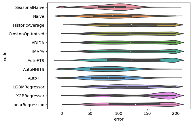 ### Choose models for groups of series
Feature:
* A unified dataframe with forecasts for all different models
* Easy Ensamble
* E.g. Average predictions
* Or MinMax (Choosing is ensembling)
```python theme={null}
# Choose the best model for each time series, metric, and cross validation window
evaluation_df['best_model'] = evaluation_df.idxmin(axis=1, numeric_only=True)
# count how many times a model wins per metric and cross validation window
count_best_model = evaluation_df.groupby(['cutoff', 'metric', 'best_model']).size().rename('n').to_frame().reset_index()
# plot results
sns.barplot(count_best_model, x='n', y='best_model', hue='metric')
```
### Choose models for groups of series
Feature:
* A unified dataframe with forecasts for all different models
* Easy Ensamble
* E.g. Average predictions
* Or MinMax (Choosing is ensembling)
```python theme={null}
# Choose the best model for each time series, metric, and cross validation window
evaluation_df['best_model'] = evaluation_df.idxmin(axis=1, numeric_only=True)
# count how many times a model wins per metric and cross validation window
count_best_model = evaluation_df.groupby(['cutoff', 'metric', 'best_model']).size().rename('n').to_frame().reset_index()
# plot results
sns.barplot(count_best_model, x='n', y='best_model', hue='metric')
```
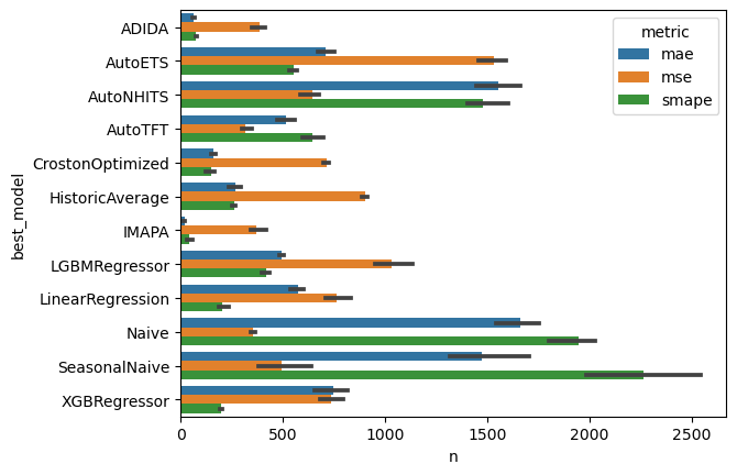 ### Et pluribus unum: an inclusive forecasting Pie.
```python theme={null}
# For the mse, calculate how many times a model wins
eval_series_df = evaluation_df.query('metric == "mse"').groupby(['unique_id']).mean(numeric_only=True)
eval_series_df['best_model'] = eval_series_df.idxmin(axis=1)
counts_series = eval_series_df.value_counts('best_model')
plt.pie(counts_series, labels=counts_series.index, autopct='%.0f%%')
plt.show()
```
### Et pluribus unum: an inclusive forecasting Pie.
```python theme={null}
# For the mse, calculate how many times a model wins
eval_series_df = evaluation_df.query('metric == "mse"').groupby(['unique_id']).mean(numeric_only=True)
eval_series_df['best_model'] = eval_series_df.idxmin(axis=1)
counts_series = eval_series_df.value_counts('best_model')
plt.pie(counts_series, labels=counts_series.index, autopct='%.0f%%')
plt.show()
```
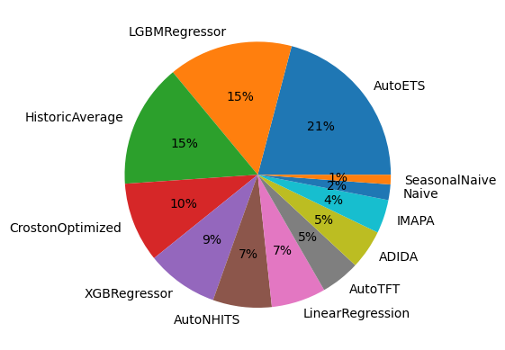 ```python theme={null}
sf.plot(Y_df, cv_df.drop(columns=['cutoff', 'y']),
max_insample_length=28 * 6,
models=['AutoNHITS'],
unique_ids=eval_series_df.query('best_model == "AutoNHITS"').index[:8])
```
# Choose Forecasting method for different groups of series
```python theme={null}
# Merge the best model per time series dataframe
# and filter the forecasts based on that dataframe
# for each time series
fcst_df = pd.melt(fcst_df.set_index('unique_id'), id_vars=['ds'], var_name='model', value_name='forecast', ignore_index=False)
fcst_df = fcst_df.join(eval_series_df[['best_model']])
fcst_df[['model', 'pred-interval']] = fcst_df['model'].str.split('-', expand=True, n=1)
fcst_df = fcst_df.query('model == best_model')
fcst_df['name'] = [f'forecast-{x}' if x is not None else 'forecast' for x in fcst_df['pred-interval']]
fcst_df = pd.pivot_table(fcst_df, index=['unique_id', 'ds'], values=['forecast'], columns=['name']).droplevel(0, axis=1).reset_index()
```
```python theme={null}
sf.plot(Y_df, fcst_df, max_insample_length=28 * 3)
```
# Technical Debt
* Train the statistical models in the full dataset.
* Increase the number of `num_samples` in the neural auto models.
* Include other models such as `Theta`, `ARIMA`, `RNN`, `LSTM`, …
# Further materials
* [Available Models StatsForecast](../../src/core/models.html)
* [Available Models
NeuralForecast](../../../neuralforecast/models.html)
* [Scalers and Loss
Functions](../../../neuralforecast/losses.pytorch.html)
* [Getting Started
NeuralForecast](../../../neuralforecast/tutorials/getting_started_complete.html)
* [Hierarchical
Reconciliation](../../../hierarchicalforecast/examples/tourismsmall.html)
* [Distributed ML Forecast
(trees)](../../../mlforecast/docs/getting-started/quick_start_distributed.html)
* [Using StatsForecast to train millions of time
series](https://www.anyscale.com/blog/how-nixtla-uses-ray-to-accurately-predict-more-than-a-million-time-series)
* [Intermittent Demand Forecasting With Nixtla on
Databricks](https://www.databricks.com/blog/2022/12/06/intermittent-demand-forecasting-nixtla-databricks.html)
```python theme={null}
sf.plot(Y_df, cv_df.drop(columns=['cutoff', 'y']),
max_insample_length=28 * 6,
models=['AutoNHITS'],
unique_ids=eval_series_df.query('best_model == "AutoNHITS"').index[:8])
```
# Choose Forecasting method for different groups of series
```python theme={null}
# Merge the best model per time series dataframe
# and filter the forecasts based on that dataframe
# for each time series
fcst_df = pd.melt(fcst_df.set_index('unique_id'), id_vars=['ds'], var_name='model', value_name='forecast', ignore_index=False)
fcst_df = fcst_df.join(eval_series_df[['best_model']])
fcst_df[['model', 'pred-interval']] = fcst_df['model'].str.split('-', expand=True, n=1)
fcst_df = fcst_df.query('model == best_model')
fcst_df['name'] = [f'forecast-{x}' if x is not None else 'forecast' for x in fcst_df['pred-interval']]
fcst_df = pd.pivot_table(fcst_df, index=['unique_id', 'ds'], values=['forecast'], columns=['name']).droplevel(0, axis=1).reset_index()
```
```python theme={null}
sf.plot(Y_df, fcst_df, max_insample_length=28 * 3)
```
# Technical Debt
* Train the statistical models in the full dataset.
* Increase the number of `num_samples` in the neural auto models.
* Include other models such as `Theta`, `ARIMA`, `RNN`, `LSTM`, …
# Further materials
* [Available Models StatsForecast](../../src/core/models.html)
* [Available Models
NeuralForecast](../../../neuralforecast/models.html)
* [Scalers and Loss
Functions](../../../neuralforecast/losses.pytorch.html)
* [Getting Started
NeuralForecast](../../../neuralforecast/tutorials/getting_started_complete.html)
* [Hierarchical
Reconciliation](../../../hierarchicalforecast/examples/tourismsmall.html)
* [Distributed ML Forecast
(trees)](../../../mlforecast/docs/getting-started/quick_start_distributed.html)
* [Using StatsForecast to train millions of time
series](https://www.anyscale.com/blog/how-nixtla-uses-ray-to-accurately-predict-more-than-a-million-time-series)
* [Intermittent Demand Forecasting With Nixtla on
Databricks](https://www.databricks.com/blog/2022/12/06/intermittent-demand-forecasting-nixtla-databricks.html)