> ## Documentation Index
> Fetch the complete documentation index at: https://nixtlaverse.nixtla.io/llms.txt
> Use this file to discover all available pages before exploring further.
# Multiple seasonalities
> In this example we will show how to forecast data with multiple
> seasonalities using an MSTL.
> **Tip**
>
> For this task, StatsForecast’s MSTL is 68% more accurate and 600%
> faster than [Prophet](https://facebook.github.io/prophet/) and
> [NeuralProphet](https://neuralprophet.com/). (Reproduce experiments
> [here](https://github.com/Nixtla/statsforecast/tree/main/experiments/mstl))
Multiple seasonal data refers to time series that have more than one
clear seasonality. Multiple seasonality is traditionally present in data
that is sampled at a low frequency. For example, hourly electricity data
exhibits daily and weekly seasonality. That means that there are clear
patterns of electricity consumption for specific hours of the day like
6:00pm vs 3:00am or for specific days like Sunday vs Friday.
Traditional statistical models are not able to model more than one
seasonal length. In this example, we will show how to model the two
seasonalities efficiently using Multiple Seasonal-Trend decompositions
with LOESS (`MSTL`).
For this example, we will use hourly electricity load data from
Pennsylvania, New Jersey, and Maryland (PJM). The original data can be
found
[here](https://github.com/jnagura/Energy-consumption-prediction-analysis).
(Click here for info on [PJM](https://www.pjm.com/about-pjm))
First, we will load the data, then we will use the `StatsForecast.fit`
and `StatsForecast.predict` methods to predict the next 24 hours. We
will then decompose the different elements of the time series into
trends and its multiple seasonalities. At the end, you will use the
`StatsForecast.forecast` for production-ready forecasting.
**Outline**
1. Install libraries
2. Load and explore the data
3. Fit a multiple-seasonality model
4. Decompose the series in trend and seasonality
5. Predict the next 24 hours
6. Optional: Forecast in production
> **Tip**
>
> You can use Colab to run this Notebook interactively
>
>
>  >
## Install libraries
We assume you have StatsForecast already installed. Check this guide for
instructions on [how to install
StatsForecast](../getting-started/installation.html).
Install the necessary packages using `pip install statsforecast`
```python theme={null}
!pip install statsforecast
```
## Load Data
The input to StatsForecast is always a data frame in [long
format](https://www.theanalysisfactor.com/wide-and-long-data/) with
three columns: `unique_id`, `ds` and `y`:
* The `unique_id` (string, int or category) represents an identifier
for the series.
* The `ds` (datestamp or int) column should be either an integer
indexing time or a datestamp ideally like YYYY-MM-DD for a date or
YYYY-MM-DD HH:MM:SS for a timestamp.
* The `y` (numeric) represents the measurement we wish to forecast. We
will rename the
You will read the data with pandas and change the necessary names. This
step should take around 2s.
```python theme={null}
import pandas as pd
```
```python theme={null}
df = pd.read_csv('https://raw.githubusercontent.com/panambY/Hourly_Energy_Consumption/master/data/PJM_Load_hourly.csv')
df.columns = ['ds', 'y']
df.insert(0, 'unique_id', 'PJM_Load_hourly')
df = df.sort_values(['unique_id', 'ds']).reset_index(drop=True)
df.tail()
```
| | unique\_id | ds | y |
| ----- | ----------------- | ------------------- | ------- |
| 32891 | PJM\_Load\_hourly | 2001-12-31 20:00:00 | 36392.0 |
| 32892 | PJM\_Load\_hourly | 2001-12-31 21:00:00 | 35082.0 |
| 32893 | PJM\_Load\_hourly | 2001-12-31 22:00:00 | 33890.0 |
| 32894 | PJM\_Load\_hourly | 2001-12-31 23:00:00 | 32590.0 |
| 32895 | PJM\_Load\_hourly | 2002-01-01 00:00:00 | 31569.0 |
StatsForecast can handle unsorted data, however, for plotting purposes,
it is convenient to sort the data frame.
Plot the series using the `plot` method from the `StatsForecast` class.
This method prints up to 8 random series from the dataset and is useful
for basic EDA. In this case, it will print just one series given that we
have just one unique\_id.
> **Note**
>
> The `StatsForecast.plot` method uses matplotlib as a default engine.
> You can change to plotly by setting `engine="plotly"`.
```python theme={null}
from statsforecast import StatsForecast
```
```python theme={null}
StatsForecast.plot(df)
```
>
## Install libraries
We assume you have StatsForecast already installed. Check this guide for
instructions on [how to install
StatsForecast](../getting-started/installation.html).
Install the necessary packages using `pip install statsforecast`
```python theme={null}
!pip install statsforecast
```
## Load Data
The input to StatsForecast is always a data frame in [long
format](https://www.theanalysisfactor.com/wide-and-long-data/) with
three columns: `unique_id`, `ds` and `y`:
* The `unique_id` (string, int or category) represents an identifier
for the series.
* The `ds` (datestamp or int) column should be either an integer
indexing time or a datestamp ideally like YYYY-MM-DD for a date or
YYYY-MM-DD HH:MM:SS for a timestamp.
* The `y` (numeric) represents the measurement we wish to forecast. We
will rename the
You will read the data with pandas and change the necessary names. This
step should take around 2s.
```python theme={null}
import pandas as pd
```
```python theme={null}
df = pd.read_csv('https://raw.githubusercontent.com/panambY/Hourly_Energy_Consumption/master/data/PJM_Load_hourly.csv')
df.columns = ['ds', 'y']
df.insert(0, 'unique_id', 'PJM_Load_hourly')
df = df.sort_values(['unique_id', 'ds']).reset_index(drop=True)
df.tail()
```
| | unique\_id | ds | y |
| ----- | ----------------- | ------------------- | ------- |
| 32891 | PJM\_Load\_hourly | 2001-12-31 20:00:00 | 36392.0 |
| 32892 | PJM\_Load\_hourly | 2001-12-31 21:00:00 | 35082.0 |
| 32893 | PJM\_Load\_hourly | 2001-12-31 22:00:00 | 33890.0 |
| 32894 | PJM\_Load\_hourly | 2001-12-31 23:00:00 | 32590.0 |
| 32895 | PJM\_Load\_hourly | 2002-01-01 00:00:00 | 31569.0 |
StatsForecast can handle unsorted data, however, for plotting purposes,
it is convenient to sort the data frame.
Plot the series using the `plot` method from the `StatsForecast` class.
This method prints up to 8 random series from the dataset and is useful
for basic EDA. In this case, it will print just one series given that we
have just one unique\_id.
> **Note**
>
> The `StatsForecast.plot` method uses matplotlib as a default engine.
> You can change to plotly by setting `engine="plotly"`.
```python theme={null}
from statsforecast import StatsForecast
```
```python theme={null}
StatsForecast.plot(df)
```
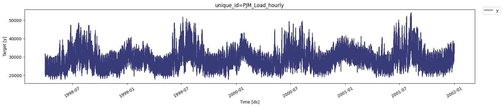 The time series exhibits seasonal patterns. Moreover, the time series
contains `32,896` observations, so it is necessary to use very
computationally efficient methods.
## Fit an MSTL model
The [MSTL](../../src/core/models.html#multipleseasonaltrend) (Multiple
Seasonal-Trend decompositions using LOESS) model, originally developed
by [Kasun Bandara, Rob J Hyndman and Christoph
Bergmeir](https://arxiv.org/abs/2107.13462), decomposes the time series
in multiple seasonalities using a Local Polynomial Regression (LOESS).
Then it forecasts the trend using a non-seasonal model and each
seasonality using a
[SeasonalNaive](../../src/core/models.html#seasonalnaive) model. You can
choose the non-seasonal model you want to use to forecast the trend
component of the MSTL model. In this example, we will use an
[AutoARIMA](../../src/core/models.html#autoarima).
Import the models you need.
```python theme={null}
from statsforecast.models import MSTL, AutoARIMA
```
First, we must define the model parameters. As mentioned before, the
electricity load presents seasonalities every 24 hours (Hourly) and
every 24 \* 7 (Daily) hours. Therefore, we will use `[24, 24 * 7]` for
season length. The trend component will be forecasted with an
`AutoARIMA` model. (You can also try with: `AutoTheta`, `AutoCES`, and
`AutoETS`)
```python theme={null}
# Create a list of models and instantiation parameters
models = [MSTL(
season_length=[24, 24 * 7], # seasonalities of the time series
trend_forecaster=AutoARIMA() # model used to forecast trend
)]
```
We fit the models by instantiating a new `StatsForecast` object with the
following required parameters:
* `models`: a list of models. Select the models you want from
[models](../../src/core/models.html) and import them.
* `freq`: a string indicating the frequency of the data. (See [panda’s
available
frequencies](https://pandas.pydata.org/pandas-docs/stable/user_guide/timeseries.html#offset-aliases).)
Any settings are passed into the constructor. Then you call its fit
method and pass in the historical data frame.
```python theme={null}
sf = StatsForecast(
models=models, # model used to fit each time series
freq='h', # frequency of the data
)
```
> **Tip**
>
> StatsForecast also supports this optional parameter.
>
> * `n_jobs`: n\_jobs: int, number of jobs used in the parallel
> processing, use -1 for all cores. (Default: 1)
>
> * `fallback_model`: a model to be used if a model fails. (Default:
> none)
Use the `fit` method to fit each model to each time series. In this
case, we are just fitting one model to one series. Check this guide to
learn how to [fit many models to many
series](../getting-started/getting_started_complete.html).
```python theme={null}
sf = sf.fit(df=df)
```
## Decompose the series
Once the model is fitted, access the decomposition using the `fitted_`
attribute of `StatsForecast`. This attribute stores all relevant
information of the fitted models for each of the time series.
In this case, we are fitting a single model for a single time series, so
by accessing the fitted\_ location \[0, 0] we will find the relevant
information of our model. The `MSTL` class generates a `model_`
attribute that contains the way the series was decomposed.
```python theme={null}
sf.fitted_[0, 0].model_
```
| | data | trend | seasonal24 | seasonal168 | remainder |
| ----- | ------- | ------------ | ------------ | ----------- | ------------ |
| 0 | 22259.0 | 25899.808157 | -4720.213546 | 581.308595 | 498.096794 |
| 1 | 21244.0 | 25900.349395 | -5433.168901 | 571.780657 | 205.038849 |
| 2 | 20651.0 | 25900.875973 | -5829.135728 | 557.142643 | 22.117112 |
| 3 | 20421.0 | 25901.387631 | -5704.092794 | 597.696957 | -373.991794 |
| 4 | 20713.0 | 25901.884103 | -5023.324375 | 922.564854 | -1088.124582 |
| ... | ... | ... | ... | ... | ... |
| 32891 | 36392.0 | 33329.031577 | 4254.112720 | 917.258336 | -2108.402633 |
| 32892 | 35082.0 | 33355.083576 | 3625.077164 | 721.689136 | -2619.849876 |
| 32893 | 33890.0 | 33381.108409 | 2571.794472 | 549.661529 | -2612.564409 |
| 32894 | 32590.0 | 33407.105839 | 796.356548 | 361.956280 | -1975.418667 |
| 32895 | 31569.0 | 33433.075723 | -1260.860917 | 279.777069 | -882.991876 |
We will use matplotlib, to visualize the different components of the
series.
```python theme={null}
import matplotlib.pyplot as plt
```
```python theme={null}
sf.fitted_[0, 0].model_.tail(24 * 28).plot(subplots=True, grid=True)
plt.tight_layout()
plt.show()
```
The time series exhibits seasonal patterns. Moreover, the time series
contains `32,896` observations, so it is necessary to use very
computationally efficient methods.
## Fit an MSTL model
The [MSTL](../../src/core/models.html#multipleseasonaltrend) (Multiple
Seasonal-Trend decompositions using LOESS) model, originally developed
by [Kasun Bandara, Rob J Hyndman and Christoph
Bergmeir](https://arxiv.org/abs/2107.13462), decomposes the time series
in multiple seasonalities using a Local Polynomial Regression (LOESS).
Then it forecasts the trend using a non-seasonal model and each
seasonality using a
[SeasonalNaive](../../src/core/models.html#seasonalnaive) model. You can
choose the non-seasonal model you want to use to forecast the trend
component of the MSTL model. In this example, we will use an
[AutoARIMA](../../src/core/models.html#autoarima).
Import the models you need.
```python theme={null}
from statsforecast.models import MSTL, AutoARIMA
```
First, we must define the model parameters. As mentioned before, the
electricity load presents seasonalities every 24 hours (Hourly) and
every 24 \* 7 (Daily) hours. Therefore, we will use `[24, 24 * 7]` for
season length. The trend component will be forecasted with an
`AutoARIMA` model. (You can also try with: `AutoTheta`, `AutoCES`, and
`AutoETS`)
```python theme={null}
# Create a list of models and instantiation parameters
models = [MSTL(
season_length=[24, 24 * 7], # seasonalities of the time series
trend_forecaster=AutoARIMA() # model used to forecast trend
)]
```
We fit the models by instantiating a new `StatsForecast` object with the
following required parameters:
* `models`: a list of models. Select the models you want from
[models](../../src/core/models.html) and import them.
* `freq`: a string indicating the frequency of the data. (See [panda’s
available
frequencies](https://pandas.pydata.org/pandas-docs/stable/user_guide/timeseries.html#offset-aliases).)
Any settings are passed into the constructor. Then you call its fit
method and pass in the historical data frame.
```python theme={null}
sf = StatsForecast(
models=models, # model used to fit each time series
freq='h', # frequency of the data
)
```
> **Tip**
>
> StatsForecast also supports this optional parameter.
>
> * `n_jobs`: n\_jobs: int, number of jobs used in the parallel
> processing, use -1 for all cores. (Default: 1)
>
> * `fallback_model`: a model to be used if a model fails. (Default:
> none)
Use the `fit` method to fit each model to each time series. In this
case, we are just fitting one model to one series. Check this guide to
learn how to [fit many models to many
series](../getting-started/getting_started_complete.html).
```python theme={null}
sf = sf.fit(df=df)
```
## Decompose the series
Once the model is fitted, access the decomposition using the `fitted_`
attribute of `StatsForecast`. This attribute stores all relevant
information of the fitted models for each of the time series.
In this case, we are fitting a single model for a single time series, so
by accessing the fitted\_ location \[0, 0] we will find the relevant
information of our model. The `MSTL` class generates a `model_`
attribute that contains the way the series was decomposed.
```python theme={null}
sf.fitted_[0, 0].model_
```
| | data | trend | seasonal24 | seasonal168 | remainder |
| ----- | ------- | ------------ | ------------ | ----------- | ------------ |
| 0 | 22259.0 | 25899.808157 | -4720.213546 | 581.308595 | 498.096794 |
| 1 | 21244.0 | 25900.349395 | -5433.168901 | 571.780657 | 205.038849 |
| 2 | 20651.0 | 25900.875973 | -5829.135728 | 557.142643 | 22.117112 |
| 3 | 20421.0 | 25901.387631 | -5704.092794 | 597.696957 | -373.991794 |
| 4 | 20713.0 | 25901.884103 | -5023.324375 | 922.564854 | -1088.124582 |
| ... | ... | ... | ... | ... | ... |
| 32891 | 36392.0 | 33329.031577 | 4254.112720 | 917.258336 | -2108.402633 |
| 32892 | 35082.0 | 33355.083576 | 3625.077164 | 721.689136 | -2619.849876 |
| 32893 | 33890.0 | 33381.108409 | 2571.794472 | 549.661529 | -2612.564409 |
| 32894 | 32590.0 | 33407.105839 | 796.356548 | 361.956280 | -1975.418667 |
| 32895 | 31569.0 | 33433.075723 | -1260.860917 | 279.777069 | -882.991876 |
We will use matplotlib, to visualize the different components of the
series.
```python theme={null}
import matplotlib.pyplot as plt
```
```python theme={null}
sf.fitted_[0, 0].model_.tail(24 * 28).plot(subplots=True, grid=True)
plt.tight_layout()
plt.show()
```
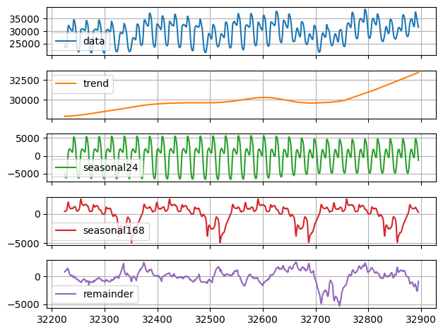 We observe a clear upward trend (orange line) and seasonality repeating
every day (24H) and every week (168H).
## Predict the next 24 hours
> Probabilistic forecasting with levels
To generate forecasts use the `predict` method.
The `predict` method takes two arguments: forecasts the next `h` (for
horizon) and `level`.
* `h` (int): represents the forecast h steps into the future. In this
case, 12 months ahead.
* `level` (list of floats): this optional parameter is used for
probabilistic forecasting. Set the `level` (or confidence
percentile) of your prediction interval. For example, `level=[90]`
means that the model expects the real value to be inside that
interval 90% of the times.
The forecast object here is a new data frame that includes a column with
the name of the model and the y hat values, as well as columns for the
uncertainty intervals.
This step should take less than 1 second.
```python theme={null}
forecasts = sf.predict(h=24, level=[90])
forecasts.head()
```
| | unique\_id | ds | MSTL | MSTL-lo-90 | MSTL-hi-90 |
| - | ----------------- | ------------------- | ------------ | ------------ | ------------ |
| 0 | PJM\_Load\_hourly | 2002-01-01 01:00:00 | 30215.608123 | 29842.185581 | 30589.030664 |
| 1 | PJM\_Load\_hourly | 2002-01-01 02:00:00 | 29447.208519 | 28787.122830 | 30107.294207 |
| 2 | PJM\_Load\_hourly | 2002-01-01 03:00:00 | 29132.786369 | 28221.353220 | 30044.219518 |
| 3 | PJM\_Load\_hourly | 2002-01-01 04:00:00 | 29126.252713 | 27992.819671 | 30259.685756 |
| 4 | PJM\_Load\_hourly | 2002-01-01 05:00:00 | 29604.606314 | 28273.426621 | 30935.786006 |
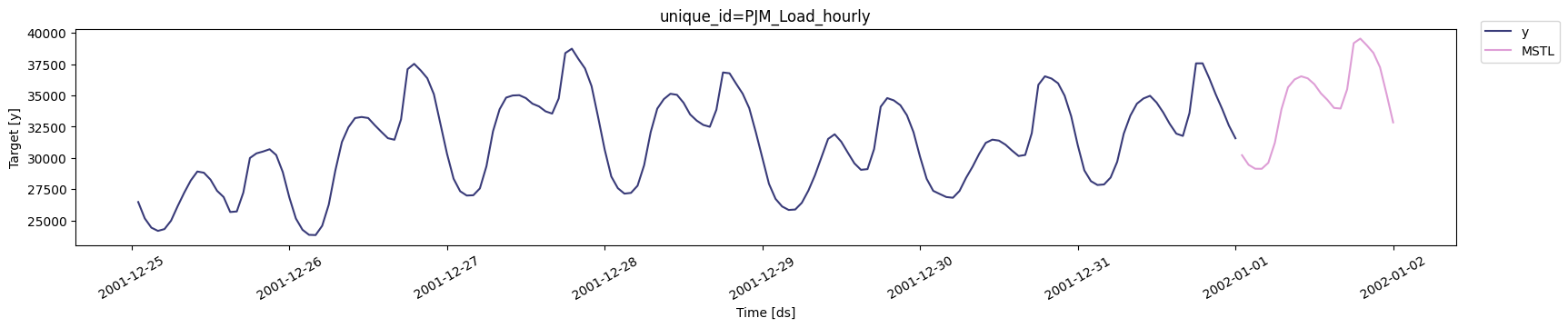
You can plot the forecast by calling the `StatsForecast.plot` method and
passing in your forecast dataframe.
```python theme={null}
sf.plot(df, forecasts, max_insample_length=24 * 7)
```
We observe a clear upward trend (orange line) and seasonality repeating
every day (24H) and every week (168H).
## Predict the next 24 hours
> Probabilistic forecasting with levels
To generate forecasts use the `predict` method.
The `predict` method takes two arguments: forecasts the next `h` (for
horizon) and `level`.
* `h` (int): represents the forecast h steps into the future. In this
case, 12 months ahead.
* `level` (list of floats): this optional parameter is used for
probabilistic forecasting. Set the `level` (or confidence
percentile) of your prediction interval. For example, `level=[90]`
means that the model expects the real value to be inside that
interval 90% of the times.
The forecast object here is a new data frame that includes a column with
the name of the model and the y hat values, as well as columns for the
uncertainty intervals.
This step should take less than 1 second.
```python theme={null}
forecasts = sf.predict(h=24, level=[90])
forecasts.head()
```
| | unique\_id | ds | MSTL | MSTL-lo-90 | MSTL-hi-90 |
| - | ----------------- | ------------------- | ------------ | ------------ | ------------ |
| 0 | PJM\_Load\_hourly | 2002-01-01 01:00:00 | 30215.608123 | 29842.185581 | 30589.030664 |
| 1 | PJM\_Load\_hourly | 2002-01-01 02:00:00 | 29447.208519 | 28787.122830 | 30107.294207 |
| 2 | PJM\_Load\_hourly | 2002-01-01 03:00:00 | 29132.786369 | 28221.353220 | 30044.219518 |
| 3 | PJM\_Load\_hourly | 2002-01-01 04:00:00 | 29126.252713 | 27992.819671 | 30259.685756 |
| 4 | PJM\_Load\_hourly | 2002-01-01 05:00:00 | 29604.606314 | 28273.426621 | 30935.786006 |
You can plot the forecast by calling the `StatsForecast.plot` method and
passing in your forecast dataframe.
```python theme={null}
sf.plot(df, forecasts, max_insample_length=24 * 7)
```
 ## Forecast in production
If you want to gain speed in productive settings where you have multiple
series or models we recommend using the `StatsForecast.forecast` method
instead of `.fit` and `.predict`.
The main difference is that the `.forecast` doest not store the fitted
values and is highly scalable in distributed environments.
The `forecast` method takes two arguments: forecasts next `h` (horizon)
and `level`.
* `h` (int): represents the forecast h steps into the future. In this
case, 12 months ahead.
* `level` (list of floats): this optional parameter is used for
probabilistic forecasting. Set the `level` (or confidence
percentile) of your prediction interval. For example, `level=[90]`
means that the model expects the real value to be inside that
interval 90% of the times.
The forecast object here is a new data frame that includes a column with
the name of the model and the y hat values, as well as columns for the
uncertainty intervals. Depending on your computer, this step should take
around 1min. (If you want to speed things up to a couple of seconds,
remove the AutoModels like ARIMA and Theta)
```python theme={null}
forecasts_df = sf.forecast(df=df, h=24, level=[90])
forecasts_df.head()
```
| | unique\_id | ds | MSTL | MSTL-lo-90 | MSTL-hi-90 |
| - | ----------------- | ------------------- | ------------ | ------------ | ------------ |
| 0 | PJM\_Load\_hourly | 2002-01-01 01:00:00 | 30215.608123 | 29842.185581 | 30589.030664 |
| 1 | PJM\_Load\_hourly | 2002-01-01 02:00:00 | 29447.208519 | 28787.122830 | 30107.294207 |
| 2 | PJM\_Load\_hourly | 2002-01-01 03:00:00 | 29132.786369 | 28221.353220 | 30044.219518 |
| 3 | PJM\_Load\_hourly | 2002-01-01 04:00:00 | 29126.252713 | 27992.819671 | 30259.685756 |
| 4 | PJM\_Load\_hourly | 2002-01-01 05:00:00 | 29604.606314 | 28273.426621 | 30935.786006 |
## References
* [Bandara, Kasun & Hyndman, Rob & Bergmeir, Christoph. (2021). “MSTL:
A Seasonal-Trend Decomposition Algorithm for Time Series with
Multiple Seasonal Patterns”](https://arxiv.org/abs/2107.13462).
## Next Steps
* Learn how to [use cross-validation to assess the robustness of your
model](../getting-started/getting_started_complete.html#evaluate-the-model%E2%80%99s-performance)
## Forecast in production
If you want to gain speed in productive settings where you have multiple
series or models we recommend using the `StatsForecast.forecast` method
instead of `.fit` and `.predict`.
The main difference is that the `.forecast` doest not store the fitted
values and is highly scalable in distributed environments.
The `forecast` method takes two arguments: forecasts next `h` (horizon)
and `level`.
* `h` (int): represents the forecast h steps into the future. In this
case, 12 months ahead.
* `level` (list of floats): this optional parameter is used for
probabilistic forecasting. Set the `level` (or confidence
percentile) of your prediction interval. For example, `level=[90]`
means that the model expects the real value to be inside that
interval 90% of the times.
The forecast object here is a new data frame that includes a column with
the name of the model and the y hat values, as well as columns for the
uncertainty intervals. Depending on your computer, this step should take
around 1min. (If you want to speed things up to a couple of seconds,
remove the AutoModels like ARIMA and Theta)
```python theme={null}
forecasts_df = sf.forecast(df=df, h=24, level=[90])
forecasts_df.head()
```
| | unique\_id | ds | MSTL | MSTL-lo-90 | MSTL-hi-90 |
| - | ----------------- | ------------------- | ------------ | ------------ | ------------ |
| 0 | PJM\_Load\_hourly | 2002-01-01 01:00:00 | 30215.608123 | 29842.185581 | 30589.030664 |
| 1 | PJM\_Load\_hourly | 2002-01-01 02:00:00 | 29447.208519 | 28787.122830 | 30107.294207 |
| 2 | PJM\_Load\_hourly | 2002-01-01 03:00:00 | 29132.786369 | 28221.353220 | 30044.219518 |
| 3 | PJM\_Load\_hourly | 2002-01-01 04:00:00 | 29126.252713 | 27992.819671 | 30259.685756 |
| 4 | PJM\_Load\_hourly | 2002-01-01 05:00:00 | 29604.606314 | 28273.426621 | 30935.786006 |
## References
* [Bandara, Kasun & Hyndman, Rob & Bergmeir, Christoph. (2021). “MSTL:
A Seasonal-Trend Decomposition Algorithm for Time Series with
Multiple Seasonal Patterns”](https://arxiv.org/abs/2107.13462).
## Next Steps
* Learn how to [use cross-validation to assess the robustness of your
model](../getting-started/getting_started_complete.html#evaluate-the-model%E2%80%99s-performance)