> ## Documentation Index
> Fetch the complete documentation index at: https://nixtlaverse.nixtla.io/llms.txt
> Use this file to discover all available pages before exploring further.
# Intermittent or Sparse Data
> In this notebook, we’ll implement models for intermittent or sparse
> data
Intermittent or sparse data has very few non-zero observations. This
type of data is hard to forecast because the zero values increase the
uncertainty about the underlying patterns in the data. Furthermore, once
a non-zero observation occurs, there can be considerable variation in
its size. Intermittent time series are common in many industries,
including finance, retail, transportation, and energy. Given the
ubiquity of this type of series, special methods have been developed to
forecast them. The first was from [Croston (1972)](#ref), followed by
several variants and by different aggregation frameworks.
[StatsForecast](../../index.html) has implemented several models to
forecast intermittent time series. By the end of this tutorial, you’ll
have a good understanding of these models and how to use them.
**Outline:**
1. Install libraries
2. Load and explore the data
3. Train models for intermittent data
4. Plot forecasts and compute accuracy
> **Tip**
>
> You can use Colab to run this Notebook interactively
>
>
>  >
> **Tip**
>
> For forecasting at scale, we recommend you check [this
> notebook](https://www.databricks.com/blog/2022/12/06/intermittent-demand-forecasting-nixtla-databricks.html)
> done on Databricks.
## Install libraries
We assume that you have StatsForecast already installed. If not, check
this guide for instructions on [how to install
StatsForecast](../getting-started/installation.html)
Install the necessary packages using `pip install statsforecast`
```python theme={null}
pip install statsforecast -U
```
## Load and explore the data
For this example, we’ll use a subset of the [M5
Competition](https://www.sciencedirect.com/science/article/pii/S0169207021001187#:~:text=The%20objective%20of%20the%20M5,the%20uncertainty%20around%20these%20forecasts)
dataset. Each time series represents the unit sales of a particular
product in a given Walmart store. At this level (product-store), most of
the data is intermittent. We first need to import the data.
```python theme={null}
import pandas as pd
```
```python theme={null}
uids = [
'FOODS_1_001_CA_1',
'FOODS_1_001_CA_2',
'FOODS_1_001_CA_3',
'FOODS_1_001_CA_4',
'FOODS_1_001_TX_1',
'FOODS_1_001_TX_2',
'FOODS_1_001_TX_3',
'FOODS_1_001_WI_1',
]
df = pd.read_parquet(
'https://datasets-nixtla.s3.amazonaws.com/m5_y.parquet',
filters=[('unique_id', 'in', uids)],
)
```
We can plot these series using the `plot_series` function from
`utilsforecast.plotting`. This function has multiple parameters, and the
required ones to generate the plots in this notebook are explained
below.
* `df`: A `pandas` dataframe with columns \[`unique_id`, `ds`, `y`].
* `forecasts_df`: A `pandas` dataframe with columns \[`unique_id`,
`ds`] and models.
* `plot_random`: Plots the time series randomly.
* `max_insample_length`: The maximum number of train/insample
observations to be plotted.
* `engine`: The library used to generate the plots. It can also be
`matplotlib` for static plots.
```python theme={null}
from utilsforecast.plotting import plot_series
```
```python theme={null}
plot_series(df, plot_random=False, max_insample_length=100)
```
>
> **Tip**
>
> For forecasting at scale, we recommend you check [this
> notebook](https://www.databricks.com/blog/2022/12/06/intermittent-demand-forecasting-nixtla-databricks.html)
> done on Databricks.
## Install libraries
We assume that you have StatsForecast already installed. If not, check
this guide for instructions on [how to install
StatsForecast](../getting-started/installation.html)
Install the necessary packages using `pip install statsforecast`
```python theme={null}
pip install statsforecast -U
```
## Load and explore the data
For this example, we’ll use a subset of the [M5
Competition](https://www.sciencedirect.com/science/article/pii/S0169207021001187#:~:text=The%20objective%20of%20the%20M5,the%20uncertainty%20around%20these%20forecasts)
dataset. Each time series represents the unit sales of a particular
product in a given Walmart store. At this level (product-store), most of
the data is intermittent. We first need to import the data.
```python theme={null}
import pandas as pd
```
```python theme={null}
uids = [
'FOODS_1_001_CA_1',
'FOODS_1_001_CA_2',
'FOODS_1_001_CA_3',
'FOODS_1_001_CA_4',
'FOODS_1_001_TX_1',
'FOODS_1_001_TX_2',
'FOODS_1_001_TX_3',
'FOODS_1_001_WI_1',
]
df = pd.read_parquet(
'https://datasets-nixtla.s3.amazonaws.com/m5_y.parquet',
filters=[('unique_id', 'in', uids)],
)
```
We can plot these series using the `plot_series` function from
`utilsforecast.plotting`. This function has multiple parameters, and the
required ones to generate the plots in this notebook are explained
below.
* `df`: A `pandas` dataframe with columns \[`unique_id`, `ds`, `y`].
* `forecasts_df`: A `pandas` dataframe with columns \[`unique_id`,
`ds`] and models.
* `plot_random`: Plots the time series randomly.
* `max_insample_length`: The maximum number of train/insample
observations to be plotted.
* `engine`: The library used to generate the plots. It can also be
`matplotlib` for static plots.
```python theme={null}
from utilsforecast.plotting import plot_series
```
```python theme={null}
plot_series(df, plot_random=False, max_insample_length=100)
```
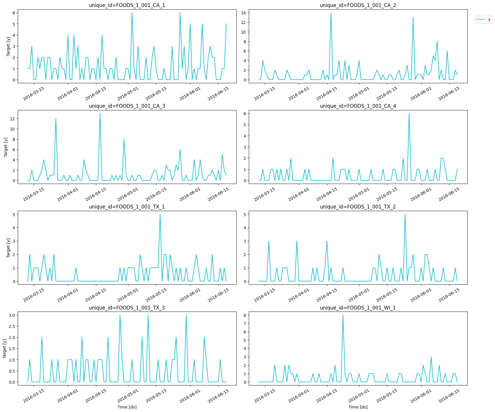 Here we only plotted the last 100 observations, but we can visualize the
complete history by removing `max_insample_length`. From these plots, we
can confirm that the data is indeed intermittent since it has multiple
periods with zero sales. In fact, in all cases but one, the median value
is zero.
```python theme={null}
df.groupby('unique_id', observed=True)['y'].median()
```
```text theme={null}
unique_id
FOODS_1_001_CA_1 0.0
FOODS_1_001_CA_2 1.0
FOODS_1_001_CA_3 0.0
FOODS_1_001_CA_4 0.0
FOODS_1_001_TX_1 0.0
FOODS_1_001_TX_2 0.0
FOODS_1_001_TX_3 0.0
FOODS_1_001_WI_1 0.0
Name: y, dtype: float32
```
## Train models for intermittent data
Before training any model, we need to separate the data in a train and a
test set. The M5 Competition used the last 28 days as test set, so we’ll
do the same.
```python theme={null}
valid_start = df['ds'].unique()[-28]
train = df[df['ds'] < valid_start]
test = df[df['ds'] >= valid_start]
```
StatsForecast has efficient implementations of multiple models for
intermittent data. The complete list of models available is
[here](../../src/core/models.html). In this notebook, we’ll use:
* [Agregate-Dissagregate Intermittent Demand Approach
(ADIDA)](../../src/core/models.html#adida)
* [Croston Classic](../../src/core/models.html#crostonclassic)
* [Intermittent Multiple Aggregation Prediction Algorithm
(IMAPA)](../../src/core/models.html#imapa)
* [Teunter-Syntetos-Babai (TSB)](../../src/core/models.html#tsb)
To use these models, we first need to import them from
`statsforecast.models` and then we need to instantiate them.
```python theme={null}
from statsforecast import StatsForecast
from statsforecast.models import (
ADIDA,
CrostonClassic,
IMAPA,
TSB
)
# Create a list of models and instantiation parameters
models = [
ADIDA(),
CrostonClassic(),
IMAPA(),
TSB(alpha_d = 0.2, alpha_p = 0.2)
]
```
To instantiate a new StatsForecast object, we need the following
parameters:
* `models`: The list of models defined in the previous step.
* `freq`: A string indicating the frequency of the data. See [pandas’
available
frequencies](https://pandas.pydata.org/pandas-docs/stable/user_guide/timeseries.html#offset-aliases).
* `n_jobs`: An integer that indicates the number of jobs used in
parallel processing. Use -1 to select all cores.
```python theme={null}
sf = StatsForecast(
models=models,
freq='D',
n_jobs=-1,
)
```
Now we’re ready to generate the forecast. To do this, we’ll use the
`forecast` method, which requires the forecasting horizon (in this case,
28 days) as argument.
The models for intermittent series that are currently available in
StatsForecast can only generate point-forecasts. If prediction intervals
are needed, then a [probabilisitic model](../../src/core/models.html)
should be used.
```python theme={null}
horizon = 28
forecasts = sf.forecast(df=train, h=horizon)
forecasts.head()
```
| | unique\_id | ds | ADIDA | CrostonClassic | IMAPA | TSB |
| - | -------------------- | ---------- | -------- | -------------- | -------- | -------- |
| 0 | FOODS\_1\_001\_CA\_1 | 2016-05-23 | 0.791852 | 0.898247 | 0.705835 | 0.434313 |
| 1 | FOODS\_1\_001\_CA\_1 | 2016-05-24 | 0.791852 | 0.898247 | 0.705835 | 0.434313 |
| 2 | FOODS\_1\_001\_CA\_1 | 2016-05-25 | 0.791852 | 0.898247 | 0.705835 | 0.434313 |
| 3 | FOODS\_1\_001\_CA\_1 | 2016-05-26 | 0.791852 | 0.898247 | 0.705835 | 0.434313 |
| 4 | FOODS\_1\_001\_CA\_1 | 2016-05-27 | 0.791852 | 0.898247 | 0.705835 | 0.434313 |
Finally, we’ll merge the forecast with the actual values.
```python theme={null}
test = test.merge(forecasts, how='left', on=['unique_id', 'ds'])
```
## Plot forecasts and compute accuracy
We can generate plots using the `plot_series` function described above.
```python theme={null}
plot_series(train, test, plot_random=False, max_insample_length=100)
```
Here we only plotted the last 100 observations, but we can visualize the
complete history by removing `max_insample_length`. From these plots, we
can confirm that the data is indeed intermittent since it has multiple
periods with zero sales. In fact, in all cases but one, the median value
is zero.
```python theme={null}
df.groupby('unique_id', observed=True)['y'].median()
```
```text theme={null}
unique_id
FOODS_1_001_CA_1 0.0
FOODS_1_001_CA_2 1.0
FOODS_1_001_CA_3 0.0
FOODS_1_001_CA_4 0.0
FOODS_1_001_TX_1 0.0
FOODS_1_001_TX_2 0.0
FOODS_1_001_TX_3 0.0
FOODS_1_001_WI_1 0.0
Name: y, dtype: float32
```
## Train models for intermittent data
Before training any model, we need to separate the data in a train and a
test set. The M5 Competition used the last 28 days as test set, so we’ll
do the same.
```python theme={null}
valid_start = df['ds'].unique()[-28]
train = df[df['ds'] < valid_start]
test = df[df['ds'] >= valid_start]
```
StatsForecast has efficient implementations of multiple models for
intermittent data. The complete list of models available is
[here](../../src/core/models.html). In this notebook, we’ll use:
* [Agregate-Dissagregate Intermittent Demand Approach
(ADIDA)](../../src/core/models.html#adida)
* [Croston Classic](../../src/core/models.html#crostonclassic)
* [Intermittent Multiple Aggregation Prediction Algorithm
(IMAPA)](../../src/core/models.html#imapa)
* [Teunter-Syntetos-Babai (TSB)](../../src/core/models.html#tsb)
To use these models, we first need to import them from
`statsforecast.models` and then we need to instantiate them.
```python theme={null}
from statsforecast import StatsForecast
from statsforecast.models import (
ADIDA,
CrostonClassic,
IMAPA,
TSB
)
# Create a list of models and instantiation parameters
models = [
ADIDA(),
CrostonClassic(),
IMAPA(),
TSB(alpha_d = 0.2, alpha_p = 0.2)
]
```
To instantiate a new StatsForecast object, we need the following
parameters:
* `models`: The list of models defined in the previous step.
* `freq`: A string indicating the frequency of the data. See [pandas’
available
frequencies](https://pandas.pydata.org/pandas-docs/stable/user_guide/timeseries.html#offset-aliases).
* `n_jobs`: An integer that indicates the number of jobs used in
parallel processing. Use -1 to select all cores.
```python theme={null}
sf = StatsForecast(
models=models,
freq='D',
n_jobs=-1,
)
```
Now we’re ready to generate the forecast. To do this, we’ll use the
`forecast` method, which requires the forecasting horizon (in this case,
28 days) as argument.
The models for intermittent series that are currently available in
StatsForecast can only generate point-forecasts. If prediction intervals
are needed, then a [probabilisitic model](../../src/core/models.html)
should be used.
```python theme={null}
horizon = 28
forecasts = sf.forecast(df=train, h=horizon)
forecasts.head()
```
| | unique\_id | ds | ADIDA | CrostonClassic | IMAPA | TSB |
| - | -------------------- | ---------- | -------- | -------------- | -------- | -------- |
| 0 | FOODS\_1\_001\_CA\_1 | 2016-05-23 | 0.791852 | 0.898247 | 0.705835 | 0.434313 |
| 1 | FOODS\_1\_001\_CA\_1 | 2016-05-24 | 0.791852 | 0.898247 | 0.705835 | 0.434313 |
| 2 | FOODS\_1\_001\_CA\_1 | 2016-05-25 | 0.791852 | 0.898247 | 0.705835 | 0.434313 |
| 3 | FOODS\_1\_001\_CA\_1 | 2016-05-26 | 0.791852 | 0.898247 | 0.705835 | 0.434313 |
| 4 | FOODS\_1\_001\_CA\_1 | 2016-05-27 | 0.791852 | 0.898247 | 0.705835 | 0.434313 |
Finally, we’ll merge the forecast with the actual values.
```python theme={null}
test = test.merge(forecasts, how='left', on=['unique_id', 'ds'])
```
## Plot forecasts and compute accuracy
We can generate plots using the `plot_series` function described above.
```python theme={null}
plot_series(train, test, plot_random=False, max_insample_length=100)
```
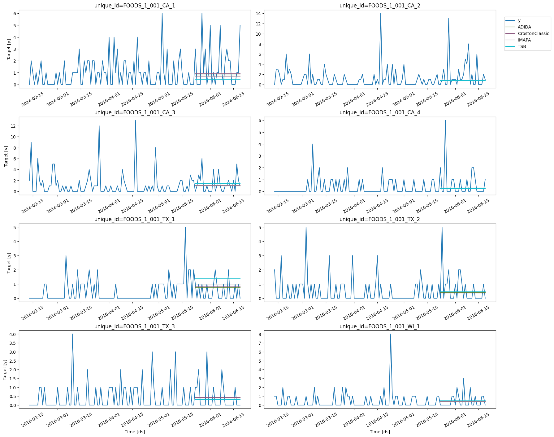 To compute the accuracy of the forecasts, we’ll use the Mean Average
Error (MAE), which is the sum of the absolute errors divided by the
number of forecasts.
```python theme={null}
from utilsforecast.evaluation import evaluate
from utilsforecast.losses import mae
```
```python theme={null}
evaluate(test, metrics=[mae], agg_fn='mean')
```
| | metric | ADIDA | CrostonClassic | IMAPA | TSB |
| - | ------ | -------- | -------------- | -------- | -------- |
| 0 | mae | 0.948729 | 0.944071 | 0.957256 | 1.023126 |
Hence, on average, the forecasts are one unit off.
## References
[Croston, J. D. (1972). Forecasting and stock control for intermittent
demands. Journal of the Operational Research Society, 23(3),
289-303.](https://link.springer.com/article/10.1057/jors.1972.50)
To compute the accuracy of the forecasts, we’ll use the Mean Average
Error (MAE), which is the sum of the absolute errors divided by the
number of forecasts.
```python theme={null}
from utilsforecast.evaluation import evaluate
from utilsforecast.losses import mae
```
```python theme={null}
evaluate(test, metrics=[mae], agg_fn='mean')
```
| | metric | ADIDA | CrostonClassic | IMAPA | TSB |
| - | ------ | -------- | -------------- | -------- | -------- |
| 0 | mae | 0.948729 | 0.944071 | 0.957256 | 1.023126 |
Hence, on average, the forecasts are one unit off.
## References
[Croston, J. D. (1972). Forecasting and stock control for intermittent
demands. Journal of the Operational Research Society, 23(3),
289-303.](https://link.springer.com/article/10.1057/jors.1972.50)