> ## Documentation Index
> Fetch the complete documentation index at: https://nixtlaverse.nixtla.io/llms.txt
> Use this file to discover all available pages before exploring further.
# Volatility forecasting (GARCH & ARCH)
> In this example, we’ll forecast the volatility of the S\&P 500 and
> several publicly traded companies using GARCH and ARCH models
> **Prerequisites**
>
> This tutorial assumes basic familiarity with StatsForecast. For a
> minimal example visit the [Quick
> Start](../getting-started/getting_started_short.html)
## Introduction
The Generalized Autoregressive Conditional Heteroskedasticity (GARCH)
model is used for time series that exhibit non-constant volatility over
time. Here volatility refers to the conditional standard deviation. The
GARCH(p,q) model is given by
where $v_t$ is independent and identically distributed with zero mean
and unit variance, and $\sigma_t$ evolves according to
The coefficients in the equation above must satisfy the following
conditions:
1. $w>0$, $\alpha_i \geq 0$ for all $i$, and $\beta_j \geq 0$ for all
$j$
2. $\sum_{k=1}^{max(p,q)} \alpha_k + \beta_k < 1$. Here it is assumed
that $\alpha_i=0$ for $i>p$ and $\beta_j=0$ for $j>q$.
A particular case of the GARCH model is the ARCH model, in which $q=0$.
Both models are commonly used in finance to model the volatility of
stock prices, exchange rates, interest rates, and other financial
instruments. They’re also used in risk management to estimate the
probability of large variations in the price of financial assets.
By the end of this tutorial, you’ll have a good understanding of how to
implement a GARCH or an ARCH model in [StatsForecast](../../index.html)
and how they can be used to analyze and predict financial time series
data.
**Outline:**
1. Install libraries
2. Load and explore the data
3. Train models
4. Perform time series cross-validation
5. Evaluate results
6. Forecast volatility
> **Tip**
>
> You can use Colab to run this Notebook interactively
>
>
>  >
## Install libraries
We assume that you have StatsForecast already installed. If not, check
this guide for instructions on [how to install
StatsForecast](../getting-started/installation.html)
Install the necessary packages using `pip install statsforecast`
```python theme={null}
%%capture
pip install statsforecast -U
```
## Load and explore the data
In this tutorial, we’ll use the last 5 years of prices from the S\&P 500
and several publicly traded companies. The data can be downloaded from
Yahoo! Finance using [yfinance](https://github.com/ranaroussi/yfinance).
To install it, use `pip install yfinance`.
```python theme={null}
%%capture
# pip install yfinance
```
We’ll also need `pandas` to deal with the dataframes.
```python theme={null}
import os
os.environ['NIXTLA_ID_AS_COL'] = '1'
import yfinance as yf
import pandas as pd
```
```python theme={null}
tickers = ['SPY', 'MSFT', 'AAPL', 'GOOG', 'AMZN', 'TSLA', 'NVDA', 'META', 'NKE', 'NFLX']
df = yf.download(tickers, start = '2018-01-01', end = '2022-12-31', interval='1mo', progress=False) # use monthly prices
df.head()
```
| Price | Adj Close | | | | | | | | | | ... | Volume | | | | | | | | | |
| ---------- | --------- | --------- | --------- | ---------- | --------- | ---------- | --------- | -------- | ---------- | --------- | --- | ---------- | ---------- | --------- | --------- | --------- | --------- | --------- | ----------- | ---------- | ---------- |
| Ticker | AAPL | AMZN | GOOG | META | MSFT | NFLX | NKE | NVDA | SPY | TSLA | ... | AAPL | AMZN | GOOG | META | MSFT | NFLX | NKE | NVDA | SPY | TSLA |
| Date | | | | | | | | | | | | | | | | | | | | | |
| 2018-01-01 | 39.388084 | 72.544502 | 58.353695 | 186.328979 | 88.027702 | 270.299988 | 63.341862 | 6.078998 | 252.565216 | 23.620667 | ... | 2638717600 | 1927424000 | 574768000 | 495655700 | 574258400 | 238377600 | 157812200 | 11456216000 | 1985506700 | 1864072500 |
| 2018-02-01 | 41.902908 | 75.622498 | 55.101181 | 177.784729 | 86.878807 | 291.380005 | 62.236938 | 5.985018 | 243.381882 | 22.870667 | ... | 3711577200 | 2755680000 | 847640000 | 516251600 | 725663300 | 184585800 | 160317000 | 14915528000 | 2923722000 | 1637850000 |
| 2018-03-01 | 39.631344 | 72.366997 | 51.463116 | 159.310333 | 84.959763 | 295.350006 | 61.689133 | 5.731123 | 235.766373 | 17.742001 | ... | 2854910800 | 2608002000 | 907066000 | 996201700 | 750754800 | 263449400 | 174066700 | 14118440000 | 2323561800 | 2359027500 |
| 2018-04-01 | 39.036106 | 78.306503 | 50.741886 | 171.483688 | 87.054207 | 312.459991 | 63.691761 | 5.565567 | 237.934006 | 19.593332 | ... | 2664617200 | 2598392000 | 834318000 | 750072700 | 668130700 | 262006000 | 158981900 | 11144008000 | 1998466500 | 2854662000 |
| 2018-05-01 | 44.140598 | 81.481003 | 54.116600 | 191.204315 | 92.006393 | 351.600006 | 66.867508 | 6.240908 | 243.717957 | 18.982000 | ... | 2483905200 | 1432310000 | 636988000 | 401144100 | 509417900 | 142050800 | 129566300 | 11978240000 | 1606397200 | 2333671500 |
The data downloaded includes different prices. We’ll use the [adjusted
closing
price](https://help.yahoo.com/kb/SLN28256.html#:~:text=Adjusted%20close%20is%20the%20closing,Security%20Prices%20\(CRSP\)%20standards.),
which is the closing price after accounting for any corporate actions
like stock splits or dividend distributions. It is also the price that
is used to examine historical returns.
Notice that the dataframe that `yfinance` returns has a
[MultiIndex](https://pandas.pydata.org/docs/user_guide/advanced.html),
so we need to select both the adjusted price and the tickers.
```python theme={null}
df = df.loc[:, (['Adj Close'], tickers)]
df.columns = df.columns.droplevel() # drop MultiIndex
df = df.reset_index()
df.head()
```
| Ticker | Date | SPY | MSFT | AAPL | GOOG | AMZN | TSLA | NVDA | META | NKE | NFLX |
| ------ | ---------- | ---------- | --------- | --------- | --------- | --------- | --------- | -------- | ---------- | --------- | ---------- |
| 0 | 2018-01-01 | 252.565216 | 88.027702 | 39.388084 | 58.353695 | 72.544502 | 23.620667 | 6.078998 | 186.328979 | 63.341862 | 270.299988 |
| 1 | 2018-02-01 | 243.381882 | 86.878807 | 41.902908 | 55.101181 | 75.622498 | 22.870667 | 5.985018 | 177.784729 | 62.236938 | 291.380005 |
| 2 | 2018-03-01 | 235.766373 | 84.959763 | 39.631344 | 51.463116 | 72.366997 | 17.742001 | 5.731123 | 159.310333 | 61.689133 | 295.350006 |
| 3 | 2018-04-01 | 237.934006 | 87.054207 | 39.036106 | 50.741886 | 78.306503 | 19.593332 | 5.565567 | 171.483688 | 63.691761 | 312.459991 |
| 4 | 2018-05-01 | 243.717957 | 92.006393 | 44.140598 | 54.116600 | 81.481003 | 18.982000 | 6.240908 | 191.204315 | 66.867508 | 351.600006 |
The input to StatsForecast is a dataframe in [long
format](https://www.theanalysisfactor.com/wide-and-long-data/) with
three columns: `unique_id`, `ds` and `y`:
* `unique_id`: (string, int or category) A unique identifier for the
series.
* `ds`: (datestamp or int) A datestamp in format YYYY-MM-DD or
YYYY-MM-DD HH:MM:SS or an integer indexing time.
* `y`: (numeric) The measurement we wish to forecast.
Hence, we need to reshape the data. We’ll do this by creating a new
dataframe called `price`.
```python theme={null}
prices = df.melt(id_vars = 'Date')
prices = prices.rename(columns={'Date': 'ds', 'Ticker': 'unique_id', 'value': 'y'})
prices = prices[['unique_id', 'ds', 'y']]
prices
```
| | unique\_id | ds | y |
| --- | ---------- | ---------- | ---------- |
| 0 | SPY | 2018-01-01 | 252.565216 |
| 1 | SPY | 2018-02-01 | 243.381882 |
| 2 | SPY | 2018-03-01 | 235.766373 |
| 3 | SPY | 2018-04-01 | 237.934006 |
| 4 | SPY | 2018-05-01 | 243.717957 |
| ... | ... | ... | ... |
| 595 | NFLX | 2022-08-01 | 223.559998 |
| 596 | NFLX | 2022-09-01 | 235.440002 |
| 597 | NFLX | 2022-10-01 | 291.880005 |
| 598 | NFLX | 2022-11-01 | 305.529999 |
| 599 | NFLX | 2022-12-01 | 294.880005 |
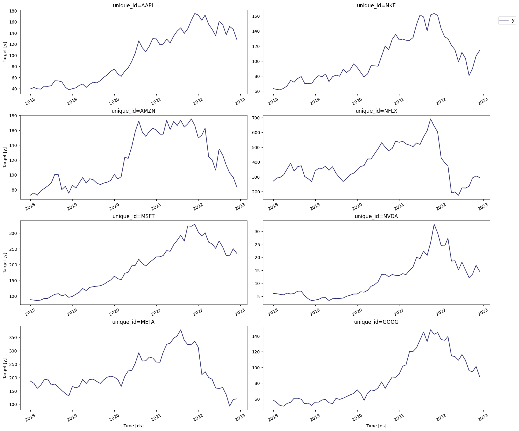
We can plot this series using the `plot` method of the StatsForecast
class.
```python theme={null}
from statsforecast import StatsForecast
```
```python theme={null}
StatsForecast.plot(prices)
```
>
## Install libraries
We assume that you have StatsForecast already installed. If not, check
this guide for instructions on [how to install
StatsForecast](../getting-started/installation.html)
Install the necessary packages using `pip install statsforecast`
```python theme={null}
%%capture
pip install statsforecast -U
```
## Load and explore the data
In this tutorial, we’ll use the last 5 years of prices from the S\&P 500
and several publicly traded companies. The data can be downloaded from
Yahoo! Finance using [yfinance](https://github.com/ranaroussi/yfinance).
To install it, use `pip install yfinance`.
```python theme={null}
%%capture
# pip install yfinance
```
We’ll also need `pandas` to deal with the dataframes.
```python theme={null}
import os
os.environ['NIXTLA_ID_AS_COL'] = '1'
import yfinance as yf
import pandas as pd
```
```python theme={null}
tickers = ['SPY', 'MSFT', 'AAPL', 'GOOG', 'AMZN', 'TSLA', 'NVDA', 'META', 'NKE', 'NFLX']
df = yf.download(tickers, start = '2018-01-01', end = '2022-12-31', interval='1mo', progress=False) # use monthly prices
df.head()
```
| Price | Adj Close | | | | | | | | | | ... | Volume | | | | | | | | | |
| ---------- | --------- | --------- | --------- | ---------- | --------- | ---------- | --------- | -------- | ---------- | --------- | --- | ---------- | ---------- | --------- | --------- | --------- | --------- | --------- | ----------- | ---------- | ---------- |
| Ticker | AAPL | AMZN | GOOG | META | MSFT | NFLX | NKE | NVDA | SPY | TSLA | ... | AAPL | AMZN | GOOG | META | MSFT | NFLX | NKE | NVDA | SPY | TSLA |
| Date | | | | | | | | | | | | | | | | | | | | | |
| 2018-01-01 | 39.388084 | 72.544502 | 58.353695 | 186.328979 | 88.027702 | 270.299988 | 63.341862 | 6.078998 | 252.565216 | 23.620667 | ... | 2638717600 | 1927424000 | 574768000 | 495655700 | 574258400 | 238377600 | 157812200 | 11456216000 | 1985506700 | 1864072500 |
| 2018-02-01 | 41.902908 | 75.622498 | 55.101181 | 177.784729 | 86.878807 | 291.380005 | 62.236938 | 5.985018 | 243.381882 | 22.870667 | ... | 3711577200 | 2755680000 | 847640000 | 516251600 | 725663300 | 184585800 | 160317000 | 14915528000 | 2923722000 | 1637850000 |
| 2018-03-01 | 39.631344 | 72.366997 | 51.463116 | 159.310333 | 84.959763 | 295.350006 | 61.689133 | 5.731123 | 235.766373 | 17.742001 | ... | 2854910800 | 2608002000 | 907066000 | 996201700 | 750754800 | 263449400 | 174066700 | 14118440000 | 2323561800 | 2359027500 |
| 2018-04-01 | 39.036106 | 78.306503 | 50.741886 | 171.483688 | 87.054207 | 312.459991 | 63.691761 | 5.565567 | 237.934006 | 19.593332 | ... | 2664617200 | 2598392000 | 834318000 | 750072700 | 668130700 | 262006000 | 158981900 | 11144008000 | 1998466500 | 2854662000 |
| 2018-05-01 | 44.140598 | 81.481003 | 54.116600 | 191.204315 | 92.006393 | 351.600006 | 66.867508 | 6.240908 | 243.717957 | 18.982000 | ... | 2483905200 | 1432310000 | 636988000 | 401144100 | 509417900 | 142050800 | 129566300 | 11978240000 | 1606397200 | 2333671500 |
The data downloaded includes different prices. We’ll use the [adjusted
closing
price](https://help.yahoo.com/kb/SLN28256.html#:~:text=Adjusted%20close%20is%20the%20closing,Security%20Prices%20\(CRSP\)%20standards.),
which is the closing price after accounting for any corporate actions
like stock splits or dividend distributions. It is also the price that
is used to examine historical returns.
Notice that the dataframe that `yfinance` returns has a
[MultiIndex](https://pandas.pydata.org/docs/user_guide/advanced.html),
so we need to select both the adjusted price and the tickers.
```python theme={null}
df = df.loc[:, (['Adj Close'], tickers)]
df.columns = df.columns.droplevel() # drop MultiIndex
df = df.reset_index()
df.head()
```
| Ticker | Date | SPY | MSFT | AAPL | GOOG | AMZN | TSLA | NVDA | META | NKE | NFLX |
| ------ | ---------- | ---------- | --------- | --------- | --------- | --------- | --------- | -------- | ---------- | --------- | ---------- |
| 0 | 2018-01-01 | 252.565216 | 88.027702 | 39.388084 | 58.353695 | 72.544502 | 23.620667 | 6.078998 | 186.328979 | 63.341862 | 270.299988 |
| 1 | 2018-02-01 | 243.381882 | 86.878807 | 41.902908 | 55.101181 | 75.622498 | 22.870667 | 5.985018 | 177.784729 | 62.236938 | 291.380005 |
| 2 | 2018-03-01 | 235.766373 | 84.959763 | 39.631344 | 51.463116 | 72.366997 | 17.742001 | 5.731123 | 159.310333 | 61.689133 | 295.350006 |
| 3 | 2018-04-01 | 237.934006 | 87.054207 | 39.036106 | 50.741886 | 78.306503 | 19.593332 | 5.565567 | 171.483688 | 63.691761 | 312.459991 |
| 4 | 2018-05-01 | 243.717957 | 92.006393 | 44.140598 | 54.116600 | 81.481003 | 18.982000 | 6.240908 | 191.204315 | 66.867508 | 351.600006 |
The input to StatsForecast is a dataframe in [long
format](https://www.theanalysisfactor.com/wide-and-long-data/) with
three columns: `unique_id`, `ds` and `y`:
* `unique_id`: (string, int or category) A unique identifier for the
series.
* `ds`: (datestamp or int) A datestamp in format YYYY-MM-DD or
YYYY-MM-DD HH:MM:SS or an integer indexing time.
* `y`: (numeric) The measurement we wish to forecast.
Hence, we need to reshape the data. We’ll do this by creating a new
dataframe called `price`.
```python theme={null}
prices = df.melt(id_vars = 'Date')
prices = prices.rename(columns={'Date': 'ds', 'Ticker': 'unique_id', 'value': 'y'})
prices = prices[['unique_id', 'ds', 'y']]
prices
```
| | unique\_id | ds | y |
| --- | ---------- | ---------- | ---------- |
| 0 | SPY | 2018-01-01 | 252.565216 |
| 1 | SPY | 2018-02-01 | 243.381882 |
| 2 | SPY | 2018-03-01 | 235.766373 |
| 3 | SPY | 2018-04-01 | 237.934006 |
| 4 | SPY | 2018-05-01 | 243.717957 |
| ... | ... | ... | ... |
| 595 | NFLX | 2022-08-01 | 223.559998 |
| 596 | NFLX | 2022-09-01 | 235.440002 |
| 597 | NFLX | 2022-10-01 | 291.880005 |
| 598 | NFLX | 2022-11-01 | 305.529999 |
| 599 | NFLX | 2022-12-01 | 294.880005 |
We can plot this series using the `plot` method of the StatsForecast
class.
```python theme={null}
from statsforecast import StatsForecast
```
```python theme={null}
StatsForecast.plot(prices)
```
 With the prices, we can compute the logarithmic returns of the S\&P 500
and the publicly traded companies. This is the variable we’re interested
in since it’s likely to work well with the GARCH framework. The
logarithmic return is given by
$return_t = log \big( \frac{price_t}{price_{t-1}} \big)$
We’ll compute the returns on the price dataframe and then we’ll create a
return dataframe with StatsForecast’s format. To do this, we’ll need
`numpy`.
```python theme={null}
import numpy as np
prices['rt'] = prices['y'].div(prices.groupby('unique_id')['y'].shift(1))
prices['rt'] = np.log(prices['rt'])
returns = prices[['unique_id', 'ds', 'rt']]
returns = returns.rename(columns={'rt':'y'})
returns
```
| | unique\_id | ds | y |
| --- | ---------- | ---------- | --------- |
| 0 | SPY | 2018-01-01 | NaN |
| 1 | SPY | 2018-02-01 | -0.037038 |
| 2 | SPY | 2018-03-01 | -0.031790 |
| 3 | SPY | 2018-04-01 | 0.009152 |
| 4 | SPY | 2018-05-01 | 0.024018 |
| ... | ... | ... | ... |
| 595 | NFLX | 2022-08-01 | -0.005976 |
| 596 | NFLX | 2022-09-01 | 0.051776 |
| 597 | NFLX | 2022-10-01 | 0.214887 |
| 598 | NFLX | 2022-11-01 | 0.045705 |
| 599 | NFLX | 2022-12-01 | -0.035479 |
> **Warning**
>
> If the order of the data is very small (say $<1e-5$),
> `scipy.optimize.minimize` might not terminate successfully. In this
> case, rescale the data and then generate the GARCH or ARCH model.
```python theme={null}
StatsForecast.plot(returns)
```
With the prices, we can compute the logarithmic returns of the S\&P 500
and the publicly traded companies. This is the variable we’re interested
in since it’s likely to work well with the GARCH framework. The
logarithmic return is given by
$return_t = log \big( \frac{price_t}{price_{t-1}} \big)$
We’ll compute the returns on the price dataframe and then we’ll create a
return dataframe with StatsForecast’s format. To do this, we’ll need
`numpy`.
```python theme={null}
import numpy as np
prices['rt'] = prices['y'].div(prices.groupby('unique_id')['y'].shift(1))
prices['rt'] = np.log(prices['rt'])
returns = prices[['unique_id', 'ds', 'rt']]
returns = returns.rename(columns={'rt':'y'})
returns
```
| | unique\_id | ds | y |
| --- | ---------- | ---------- | --------- |
| 0 | SPY | 2018-01-01 | NaN |
| 1 | SPY | 2018-02-01 | -0.037038 |
| 2 | SPY | 2018-03-01 | -0.031790 |
| 3 | SPY | 2018-04-01 | 0.009152 |
| 4 | SPY | 2018-05-01 | 0.024018 |
| ... | ... | ... | ... |
| 595 | NFLX | 2022-08-01 | -0.005976 |
| 596 | NFLX | 2022-09-01 | 0.051776 |
| 597 | NFLX | 2022-10-01 | 0.214887 |
| 598 | NFLX | 2022-11-01 | 0.045705 |
| 599 | NFLX | 2022-12-01 | -0.035479 |
> **Warning**
>
> If the order of the data is very small (say $<1e-5$),
> `scipy.optimize.minimize` might not terminate successfully. In this
> case, rescale the data and then generate the GARCH or ARCH model.
```python theme={null}
StatsForecast.plot(returns)
```
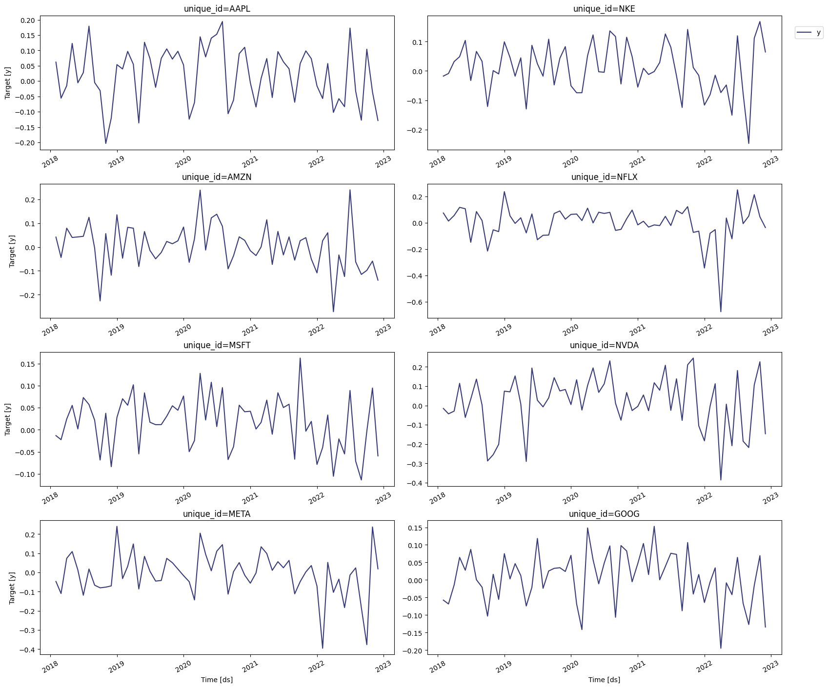 From this plot, we can see that the returns seem suited for the GARCH
framework, since large shocks *tend* to be followed by other large
shocks. This doesn’t mean that after every large shock we should expect
another one; merely that the probability of a large variance is greater
than the probability of a small one.
## Train models
We first need to import the
[GARCH](../../src/core/models.html#GARCH.html) and the
[ARCH](../../src/core/models.html#ARCH.html) models from
`statsforecast.models`, and then we need to fit them by instantiating a
new StatsForecast object. Notice that we’ll be using different values of
$p$ and $q$. In the next section, we’ll determine which ones produce the
most accurate model using cross-validation. We’ll also import the
[Naive](../../src/core/models.html#naive) model since we’ll use it as a
baseline.
```python theme={null}
from statsforecast.models import (
GARCH,
ARCH,
Naive
)
models = [ARCH(1),
ARCH(2),
GARCH(1,1),
GARCH(1,2),
GARCH(2,2),
GARCH(2,1),
Naive()
]
```
To instantiate a new StatsForecast object, we need the following
parameters:
* `df`: The dataframe with the training data.
* `models`: The list of models defined in the previous step.
* `freq`: A string indicating the frequency of the data. Here we’ll
use **MS**, which correspond to the start of the month. You can see
the list of panda’s available frequencies
[here](https://pandas.pydata.org/pandas-docs/stable/user_guide/timeseries.html#offset-aliases).
* `n_jobs`: An integer that indicates the number of jobs used in
parallel processing. Use -1 to select all cores.
```python theme={null}
sf = StatsForecast(
models = models,
freq = 'MS',
n_jobs = -1
)
```
## Perform time series cross-validation
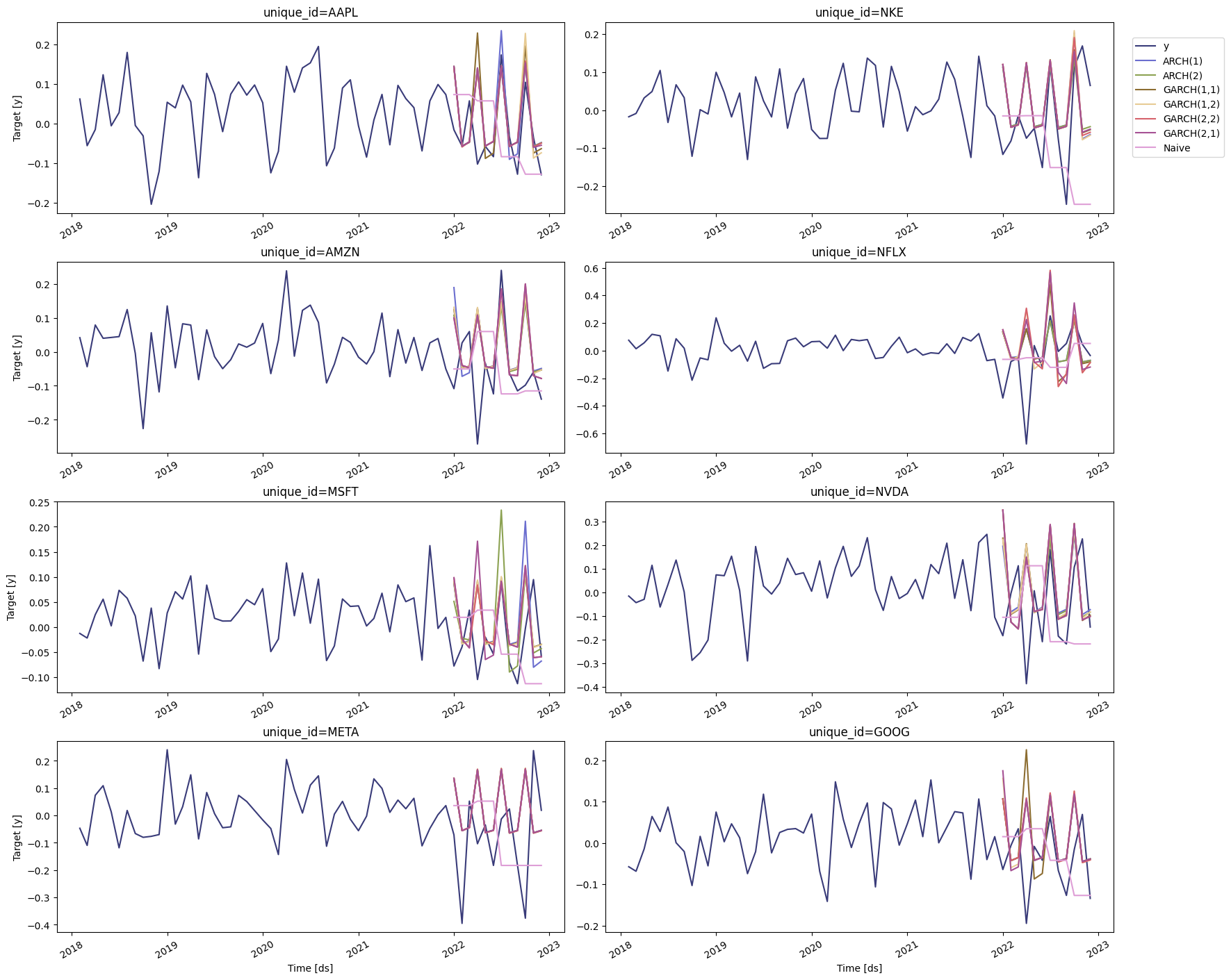
Time series cross-validation is a method for evaluating how a model
would have performed in the past. It works by defining a sliding window
across the historical data and predicting the period following it. Here
we’ll use StatsForecast’s `cross-validation` method to determine the
most accurate model for the S\&P 500 and the companies selected.
This method takes the following arguments:
* `df`: The dataframe with the training data.
* `h` (int): represents the h steps into the future that will be
forecasted.
* `step_size` (int): step size between each window, meaning how often
do you want to run the forecasting process.
* `n_windows` (int): number of windows used for cross-validation,
meaning the number of forecasting processes in the past you want to
evaluate.
For this particular example, we’ll use 4 windows of 3 months, or all the
quarters in a year.
```python theme={null}
cv_df = sf.cross_validation(
df = returns,
h = 3,
step_size = 3,
n_windows = 4
)
```
The `cv_df` object is a dataframe with the following columns:
* `unique_id`: series identifier.
* `ds`: datestamp or temporal index
* `cutoff`: the last datestamp or temporal index for the `n_windows`.
* `y`: true value
* `"model"`: columns with the model’s name and fitted value.
```python theme={null}
cv_df.rename(columns = {'y' : 'actual'}, inplace = True)
cv_df.head()
```
| | unique\_id | ds | cutoff | actual | ARCH(1) | ARCH(2) | GARCH(1,1) | GARCH(1,2) | GARCH(2,2) | GARCH(2,1) | Naive |
| - | ---------- | ---------- | ---------- | --------- | --------- | --------- | ---------- | ---------- | ---------- | ---------- | -------- |
| 0 | AAPL | 2022-01-01 | 2021-12-01 | -0.015837 | 0.142421 | 0.144016 | 0.142954 | 0.141682 | 0.141682 | 0.144015 | 0.073061 |
| 1 | AAPL | 2022-02-01 | 2021-12-01 | -0.056856 | -0.056893 | -0.057158 | -0.056388 | -0.058786 | -0.058785 | -0.057158 | 0.073061 |
| 2 | AAPL | 2022-03-01 | 2021-12-01 | 0.057156 | -0.045901 | -0.046479 | -0.047513 | -0.045711 | -0.045711 | -0.046478 | 0.073061 |
| 3 | AAPL | 2022-04-01 | 2022-03-01 | -0.102178 | 0.138650 | 0.140222 | 0.228138 | 0.136118 | 0.136132 | 0.140211 | 0.057156 |
| 4 | AAPL | 2022-05-01 | 2022-03-01 | -0.057505 | -0.056007 | -0.056268 | -0.087833 | -0.057078 | -0.057085 | -0.056265 | 0.057156 |
```python theme={null}
StatsForecast.plot(returns, cv_df.drop(['cutoff', 'actual'], axis=1))
```
From this plot, we can see that the returns seem suited for the GARCH
framework, since large shocks *tend* to be followed by other large
shocks. This doesn’t mean that after every large shock we should expect
another one; merely that the probability of a large variance is greater
than the probability of a small one.
## Train models
We first need to import the
[GARCH](../../src/core/models.html#GARCH.html) and the
[ARCH](../../src/core/models.html#ARCH.html) models from
`statsforecast.models`, and then we need to fit them by instantiating a
new StatsForecast object. Notice that we’ll be using different values of
$p$ and $q$. In the next section, we’ll determine which ones produce the
most accurate model using cross-validation. We’ll also import the
[Naive](../../src/core/models.html#naive) model since we’ll use it as a
baseline.
```python theme={null}
from statsforecast.models import (
GARCH,
ARCH,
Naive
)
models = [ARCH(1),
ARCH(2),
GARCH(1,1),
GARCH(1,2),
GARCH(2,2),
GARCH(2,1),
Naive()
]
```
To instantiate a new StatsForecast object, we need the following
parameters:
* `df`: The dataframe with the training data.
* `models`: The list of models defined in the previous step.
* `freq`: A string indicating the frequency of the data. Here we’ll
use **MS**, which correspond to the start of the month. You can see
the list of panda’s available frequencies
[here](https://pandas.pydata.org/pandas-docs/stable/user_guide/timeseries.html#offset-aliases).
* `n_jobs`: An integer that indicates the number of jobs used in
parallel processing. Use -1 to select all cores.
```python theme={null}
sf = StatsForecast(
models = models,
freq = 'MS',
n_jobs = -1
)
```
## Perform time series cross-validation
Time series cross-validation is a method for evaluating how a model
would have performed in the past. It works by defining a sliding window
across the historical data and predicting the period following it. Here
we’ll use StatsForecast’s `cross-validation` method to determine the
most accurate model for the S\&P 500 and the companies selected.
This method takes the following arguments:
* `df`: The dataframe with the training data.
* `h` (int): represents the h steps into the future that will be
forecasted.
* `step_size` (int): step size between each window, meaning how often
do you want to run the forecasting process.
* `n_windows` (int): number of windows used for cross-validation,
meaning the number of forecasting processes in the past you want to
evaluate.
For this particular example, we’ll use 4 windows of 3 months, or all the
quarters in a year.
```python theme={null}
cv_df = sf.cross_validation(
df = returns,
h = 3,
step_size = 3,
n_windows = 4
)
```
The `cv_df` object is a dataframe with the following columns:
* `unique_id`: series identifier.
* `ds`: datestamp or temporal index
* `cutoff`: the last datestamp or temporal index for the `n_windows`.
* `y`: true value
* `"model"`: columns with the model’s name and fitted value.
```python theme={null}
cv_df.rename(columns = {'y' : 'actual'}, inplace = True)
cv_df.head()
```
| | unique\_id | ds | cutoff | actual | ARCH(1) | ARCH(2) | GARCH(1,1) | GARCH(1,2) | GARCH(2,2) | GARCH(2,1) | Naive |
| - | ---------- | ---------- | ---------- | --------- | --------- | --------- | ---------- | ---------- | ---------- | ---------- | -------- |
| 0 | AAPL | 2022-01-01 | 2021-12-01 | -0.015837 | 0.142421 | 0.144016 | 0.142954 | 0.141682 | 0.141682 | 0.144015 | 0.073061 |
| 1 | AAPL | 2022-02-01 | 2021-12-01 | -0.056856 | -0.056893 | -0.057158 | -0.056388 | -0.058786 | -0.058785 | -0.057158 | 0.073061 |
| 2 | AAPL | 2022-03-01 | 2021-12-01 | 0.057156 | -0.045901 | -0.046479 | -0.047513 | -0.045711 | -0.045711 | -0.046478 | 0.073061 |
| 3 | AAPL | 2022-04-01 | 2022-03-01 | -0.102178 | 0.138650 | 0.140222 | 0.228138 | 0.136118 | 0.136132 | 0.140211 | 0.057156 |
| 4 | AAPL | 2022-05-01 | 2022-03-01 | -0.057505 | -0.056007 | -0.056268 | -0.087833 | -0.057078 | -0.057085 | -0.056265 | 0.057156 |
```python theme={null}
StatsForecast.plot(returns, cv_df.drop(['cutoff', 'actual'], axis=1))
```
 A tutorial on cross-validation can be found
[here](./crossvalidation.html)
## Evaluate results
To compute the accuracy of the forecasts, we’ll use the mean average
error (mae), which is the sum of the absolute errors divided by the
number of forecasts.
```python theme={null}
from utilsforecast.evaluation import evaluate
from utilsforecast.losses import mae
```
The MAE needs to be computed for every window and then it needs to be
averaged across all of them. To do this, we’ll create the following
function.
```python theme={null}
models = cv_df.columns.drop(['unique_id', 'ds', 'cutoff', 'actual'])
```
```python theme={null}
mae_cv = evaluate(cv_df, metrics=[mae], models=models, target_col='actual')
mae_cv = mae_cv.drop(columns=['metric']).set_index('unique_id')
mae_cv
```
| | ARCH(1) | ARCH(2) | GARCH(1,1) | GARCH(1,2) | GARCH(2,2) | GARCH(2,1) | Naive |
| ---------- | -------- | -------- | ---------- | ---------- | ---------- | ---------- | -------- |
| unique\_id | | | | | | | |
| AAPL | 0.071773 | 0.068927 | 0.080182 | 0.075321 | 0.069187 | 0.068817 | 0.110426 |
| AMZN | 0.127390 | 0.113613 | 0.118859 | 0.119930 | 0.109910 | 0.109910 | 0.115189 |
| GOOG | 0.093849 | 0.093753 | 0.109662 | 0.101583 | 0.094648 | 0.103389 | 0.083233 |
| META | 0.198334 | 0.198893 | 0.199615 | 0.199711 | 0.199712 | 0.198892 | 0.185346 |
| MSFT | 0.082373 | 0.075055 | 0.072241 | 0.072765 | 0.073006 | 0.082066 | 0.086951 |
| NFLX | 0.159386 | 0.159528 | 0.199623 | 0.232477 | 0.230075 | 0.230770 | 0.167421 |
| NKE | 0.108337 | 0.098918 | 0.103366 | 0.110278 | 0.107179 | 0.102708 | 0.160404 |
| NVDA | 0.189461 | 0.207871 | 0.198999 | 0.196170 | 0.211932 | 0.211940 | 0.215289 |
| SPY | 0.058511 | 0.058583 | 0.058701 | 0.062492 | 0.057053 | 0.068192 | 0.089012 |
| TSLA | 0.192003 | 0.192618 | 0.190225 | 0.192354 | 0.191620 | 0.191423 | 0.218857 |
```python theme={null}
mae_cv.idxmin(axis=1)
```
```text theme={null}
unique_id
AAPL GARCH(2,1)
AMZN GARCH(2,2)
GOOG Naive
META Naive
MSFT GARCH(1,1)
NFLX ARCH(1)
NKE ARCH(2)
NVDA ARCH(1)
SPY GARCH(2,2)
TSLA GARCH(1,1)
dtype: object
```
Hence, the most accurate model to describe the logarithmic returns of
Apple’s stock is a GARCH(2, 1), for Amazon’s stock is a GARCH(2,2), and
so on.
## Forecast volatility
We can now generate a forecast for the next quarter. To do this, we’ll
use the `forecast` method, which requires the following arguments:
* `h`: (int) The forecasting horizon.
* `level`: (list\[float]) The confidence levels of the prediction
intervals
* `fitted` : (bool = False) Returns insample predictions.
```python theme={null}
levels = [80, 95] # confidence levels for the prediction intervals
forecasts = sf.forecast(df=returns, h=3, level=levels)
forecasts.head()
```
| | unique\_id | ds | ARCH(1) | ARCH(1)-lo-95 | ARCH(1)-lo-80 | ARCH(1)-hi-80 | ARCH(1)-hi-95 | ARCH(2) | ARCH(2)-lo-95 | ARCH(2)-lo-80 | ... | GARCH(2,1) | GARCH(2,1)-lo-95 | GARCH(2,1)-lo-80 | GARCH(2,1)-hi-80 | GARCH(2,1)-hi-95 | Naive | Naive-lo-80 | Naive-lo-95 | Naive-hi-80 | Naive-hi-95 |
| - | ---------- | ---------- | --------- | ------------- | ------------- | ------------- | ------------- | --------- | ------------- | ------------- | --- | ---------- | ---------------- | ---------------- | ---------------- | ---------------- | --------- | ----------- | ----------- | ----------- | ----------- |
| 0 | AAPL | 2023-01-01 | 0.150457 | 0.133641 | 0.139462 | 0.161453 | 0.167273 | 0.150158 | 0.133409 | 0.139206 | ... | 0.147602 | 0.131418 | 0.137020 | 0.158184 | 0.163786 | -0.128762 | -0.284462 | -0.366885 | 0.026939 | 0.109362 |
| 1 | AAPL | 2023-02-01 | -0.056943 | -0.073924 | -0.068046 | -0.045839 | -0.039961 | -0.057207 | -0.074346 | -0.068414 | ... | -0.059512 | -0.078060 | -0.071640 | -0.047384 | -0.040964 | -0.128762 | -0.348956 | -0.465520 | 0.091433 | 0.207997 |
| 2 | AAPL | 2023-03-01 | -0.048391 | -0.064843 | -0.059148 | -0.037633 | -0.031939 | -0.049282 | -0.066345 | -0.060439 | ... | -0.054539 | -0.075438 | -0.068204 | -0.040875 | -0.033641 | -0.128762 | -0.398443 | -0.541204 | 0.140920 | 0.283681 |
| 3 | AMZN | 2023-01-01 | 0.152147 | 0.134952 | 0.140904 | 0.163391 | 0.169343 | 0.148658 | 0.132242 | 0.137924 | ... | 0.148599 | 0.132196 | 0.137873 | 0.159324 | 0.165001 | -0.139141 | -0.315716 | -0.409190 | 0.037435 | 0.130909 |
| 4 | AMZN | 2023-02-01 | -0.057301 | -0.074497 | -0.068545 | -0.046058 | -0.040106 | -0.061187 | -0.080794 | -0.074007 | ... | -0.069303 | -0.094457 | -0.085750 | -0.052856 | -0.044150 | -0.139141 | -0.388856 | -0.521048 | 0.110575 | 0.242767 |
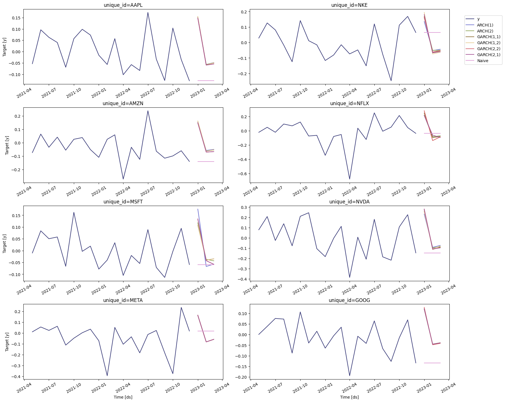
With the results of the previous section, we can choose the best model
for the S\&P 500 and the companies selected. Some of the plots are shown
below. Notice that we’re using some additional arguments in the `plot`
method:
* `level`: (list\[int]) The confidence levels for the prediction
intervals (this was already defined).
* `unique_ids`: (list\[str, int or category]) The ids to plot.
* `models`: (list(str)). The model to plot. In this case, is the model
selected by cross-validation.
```python theme={null}
StatsForecast.plot(returns, forecasts, max_insample_length=20)
```
A tutorial on cross-validation can be found
[here](./crossvalidation.html)
## Evaluate results
To compute the accuracy of the forecasts, we’ll use the mean average
error (mae), which is the sum of the absolute errors divided by the
number of forecasts.
```python theme={null}
from utilsforecast.evaluation import evaluate
from utilsforecast.losses import mae
```
The MAE needs to be computed for every window and then it needs to be
averaged across all of them. To do this, we’ll create the following
function.
```python theme={null}
models = cv_df.columns.drop(['unique_id', 'ds', 'cutoff', 'actual'])
```
```python theme={null}
mae_cv = evaluate(cv_df, metrics=[mae], models=models, target_col='actual')
mae_cv = mae_cv.drop(columns=['metric']).set_index('unique_id')
mae_cv
```
| | ARCH(1) | ARCH(2) | GARCH(1,1) | GARCH(1,2) | GARCH(2,2) | GARCH(2,1) | Naive |
| ---------- | -------- | -------- | ---------- | ---------- | ---------- | ---------- | -------- |
| unique\_id | | | | | | | |
| AAPL | 0.071773 | 0.068927 | 0.080182 | 0.075321 | 0.069187 | 0.068817 | 0.110426 |
| AMZN | 0.127390 | 0.113613 | 0.118859 | 0.119930 | 0.109910 | 0.109910 | 0.115189 |
| GOOG | 0.093849 | 0.093753 | 0.109662 | 0.101583 | 0.094648 | 0.103389 | 0.083233 |
| META | 0.198334 | 0.198893 | 0.199615 | 0.199711 | 0.199712 | 0.198892 | 0.185346 |
| MSFT | 0.082373 | 0.075055 | 0.072241 | 0.072765 | 0.073006 | 0.082066 | 0.086951 |
| NFLX | 0.159386 | 0.159528 | 0.199623 | 0.232477 | 0.230075 | 0.230770 | 0.167421 |
| NKE | 0.108337 | 0.098918 | 0.103366 | 0.110278 | 0.107179 | 0.102708 | 0.160404 |
| NVDA | 0.189461 | 0.207871 | 0.198999 | 0.196170 | 0.211932 | 0.211940 | 0.215289 |
| SPY | 0.058511 | 0.058583 | 0.058701 | 0.062492 | 0.057053 | 0.068192 | 0.089012 |
| TSLA | 0.192003 | 0.192618 | 0.190225 | 0.192354 | 0.191620 | 0.191423 | 0.218857 |
```python theme={null}
mae_cv.idxmin(axis=1)
```
```text theme={null}
unique_id
AAPL GARCH(2,1)
AMZN GARCH(2,2)
GOOG Naive
META Naive
MSFT GARCH(1,1)
NFLX ARCH(1)
NKE ARCH(2)
NVDA ARCH(1)
SPY GARCH(2,2)
TSLA GARCH(1,1)
dtype: object
```
Hence, the most accurate model to describe the logarithmic returns of
Apple’s stock is a GARCH(2, 1), for Amazon’s stock is a GARCH(2,2), and
so on.
## Forecast volatility
We can now generate a forecast for the next quarter. To do this, we’ll
use the `forecast` method, which requires the following arguments:
* `h`: (int) The forecasting horizon.
* `level`: (list\[float]) The confidence levels of the prediction
intervals
* `fitted` : (bool = False) Returns insample predictions.
```python theme={null}
levels = [80, 95] # confidence levels for the prediction intervals
forecasts = sf.forecast(df=returns, h=3, level=levels)
forecasts.head()
```
| | unique\_id | ds | ARCH(1) | ARCH(1)-lo-95 | ARCH(1)-lo-80 | ARCH(1)-hi-80 | ARCH(1)-hi-95 | ARCH(2) | ARCH(2)-lo-95 | ARCH(2)-lo-80 | ... | GARCH(2,1) | GARCH(2,1)-lo-95 | GARCH(2,1)-lo-80 | GARCH(2,1)-hi-80 | GARCH(2,1)-hi-95 | Naive | Naive-lo-80 | Naive-lo-95 | Naive-hi-80 | Naive-hi-95 |
| - | ---------- | ---------- | --------- | ------------- | ------------- | ------------- | ------------- | --------- | ------------- | ------------- | --- | ---------- | ---------------- | ---------------- | ---------------- | ---------------- | --------- | ----------- | ----------- | ----------- | ----------- |
| 0 | AAPL | 2023-01-01 | 0.150457 | 0.133641 | 0.139462 | 0.161453 | 0.167273 | 0.150158 | 0.133409 | 0.139206 | ... | 0.147602 | 0.131418 | 0.137020 | 0.158184 | 0.163786 | -0.128762 | -0.284462 | -0.366885 | 0.026939 | 0.109362 |
| 1 | AAPL | 2023-02-01 | -0.056943 | -0.073924 | -0.068046 | -0.045839 | -0.039961 | -0.057207 | -0.074346 | -0.068414 | ... | -0.059512 | -0.078060 | -0.071640 | -0.047384 | -0.040964 | -0.128762 | -0.348956 | -0.465520 | 0.091433 | 0.207997 |
| 2 | AAPL | 2023-03-01 | -0.048391 | -0.064843 | -0.059148 | -0.037633 | -0.031939 | -0.049282 | -0.066345 | -0.060439 | ... | -0.054539 | -0.075438 | -0.068204 | -0.040875 | -0.033641 | -0.128762 | -0.398443 | -0.541204 | 0.140920 | 0.283681 |
| 3 | AMZN | 2023-01-01 | 0.152147 | 0.134952 | 0.140904 | 0.163391 | 0.169343 | 0.148658 | 0.132242 | 0.137924 | ... | 0.148599 | 0.132196 | 0.137873 | 0.159324 | 0.165001 | -0.139141 | -0.315716 | -0.409190 | 0.037435 | 0.130909 |
| 4 | AMZN | 2023-02-01 | -0.057301 | -0.074497 | -0.068545 | -0.046058 | -0.040106 | -0.061187 | -0.080794 | -0.074007 | ... | -0.069303 | -0.094457 | -0.085750 | -0.052856 | -0.044150 | -0.139141 | -0.388856 | -0.521048 | 0.110575 | 0.242767 |
With the results of the previous section, we can choose the best model
for the S\&P 500 and the companies selected. Some of the plots are shown
below. Notice that we’re using some additional arguments in the `plot`
method:
* `level`: (list\[int]) The confidence levels for the prediction
intervals (this was already defined).
* `unique_ids`: (list\[str, int or category]) The ids to plot.
* `models`: (list(str)). The model to plot. In this case, is the model
selected by cross-validation.
```python theme={null}
StatsForecast.plot(returns, forecasts, max_insample_length=20)
```
 ## References
* [Engle, R. F. (1982). Autoregressive conditional heteroscedasticity
with estimates of the variance of United Kingdom inflation.
Econometrica: Journal of the econometric society,
987-1007.](http://www.econ.uiuc.edu/~econ508/Papers/engle82.pdf)
* [Bollerslev, T. (1986). Generalized autoregressive conditional
heteroskedasticity. Journal of econometrics, 31(3),
307-327.](https://citeseerx.ist.psu.edu/document?repid=rep1\&type=pdf\&doi=7da8bfa5295375c1141d797e80065a599153c19d)
* [Hamilton, J. D. (1994). Time series analysis. Princeton university
press.](https://press.princeton.edu/books/hardcover/9780691042893/time-series-analysis)
* [Tsay, R. S. (2005). Analysis of financial time series. John wiley &
sons.](https://www.wiley.com/en-us/Analysis+of+Financial+Time+Series%2C+3rd+Edition-p-9780470414354)
## References
* [Engle, R. F. (1982). Autoregressive conditional heteroscedasticity
with estimates of the variance of United Kingdom inflation.
Econometrica: Journal of the econometric society,
987-1007.](http://www.econ.uiuc.edu/~econ508/Papers/engle82.pdf)
* [Bollerslev, T. (1986). Generalized autoregressive conditional
heteroskedasticity. Journal of econometrics, 31(3),
307-327.](https://citeseerx.ist.psu.edu/document?repid=rep1\&type=pdf\&doi=7da8bfa5295375c1141d797e80065a599153c19d)
* [Hamilton, J. D. (1994). Time series analysis. Princeton university
press.](https://press.princeton.edu/books/hardcover/9780691042893/time-series-analysis)
* [Tsay, R. S. (2005). Analysis of financial time series. John wiley &
sons.](https://www.wiley.com/en-us/Analysis+of+Financial+Time+Series%2C+3rd+Edition-p-9780470414354)