> ## Documentation Index
> Fetch the complete documentation index at: https://nixtlaverse.nixtla.io/llms.txt
> Use this file to discover all available pages before exploring further.
# MFLES
> MFLES is a simple time series method based on gradient boosting time
> series decomposition.
There are numerous methods that can enter the boosting loop depending on
user-provided parameters or some quick logic MFLES does automatically
that seems to work ok. Some of these methods are:
1. SES Ensemble
2. Simple Moving Average
3. Piecewise Linear Trend
4. Fourier Basis function regression for seasonality
5. Simple Median
6. A Robust Linear Method for trend
# **Gradient Boosted Decomposition**
This approach aims to view a time series decomposition (trend,
seasonality, and exogenous) as the ‘weak’ estimator in a gradient
boosting procedure.
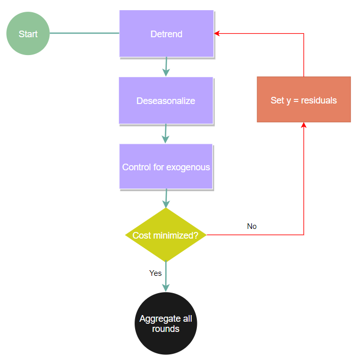 The major relevant changes to note are:
1. The trend estimator will always go from simple to complex. Beginning
with a median, then to a linear/piecewise linear, then to some sort
of smoother.
2. Multiple seasonality is fit one seasonality per boosting round
rather than simultaneously. This means you should organize your
seasonality in order of perceived importance. Also, theoretically,
you can have up to 50 seasonalities present by default, but after 3
you should expect degraded performance.
3. Learning rates are now estimator specific rather than a single
parameter like you would see in something like XGBoost. This is
useful if you have exogenous signals that are also seasonal, you
(this will not be done automatically) can optimize for the
combination of the seasonal signal and the exogenous signal.
# **Let’s forecast**
```python theme={null}
# %pip install statsforecast
```
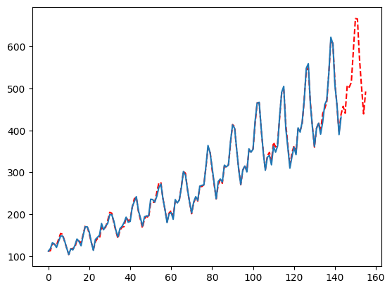
Here, we will use the specific model object in Statsforecast and the
infamous airline passengers dataset 😀:
```python theme={null}
import pandas as pd
import numpy as np
from statsforecast.models import AutoMFLES
import matplotlib.pyplot as plt
df = pd.read_csv(r'https://raw.githubusercontent.com/jbrownlee/Datasets/master/airline-passengers.csv')
y = df['Passengers'].values # make array
mfles_model = AutoMFLES(
season_length = [12],
test_size = 12,
n_windows=2,
metric = 'smape')
mfles_model.fit(y=y)
predicted = mfles_model.predict(12)['mean']
fitted = mfles_model.predict_in_sample()['fitted']
```
```python theme={null}
plt.plot(np.append(fitted, predicted), linestyle='dashed', color='red')
plt.plot(y)
plt.show()
```
The major relevant changes to note are:
1. The trend estimator will always go from simple to complex. Beginning
with a median, then to a linear/piecewise linear, then to some sort
of smoother.
2. Multiple seasonality is fit one seasonality per boosting round
rather than simultaneously. This means you should organize your
seasonality in order of perceived importance. Also, theoretically,
you can have up to 50 seasonalities present by default, but after 3
you should expect degraded performance.
3. Learning rates are now estimator specific rather than a single
parameter like you would see in something like XGBoost. This is
useful if you have exogenous signals that are also seasonal, you
(this will not be done automatically) can optimize for the
combination of the seasonal signal and the exogenous signal.
# **Let’s forecast**
```python theme={null}
# %pip install statsforecast
```
Here, we will use the specific model object in Statsforecast and the
infamous airline passengers dataset 😀:
```python theme={null}
import pandas as pd
import numpy as np
from statsforecast.models import AutoMFLES
import matplotlib.pyplot as plt
df = pd.read_csv(r'https://raw.githubusercontent.com/jbrownlee/Datasets/master/airline-passengers.csv')
y = df['Passengers'].values # make array
mfles_model = AutoMFLES(
season_length = [12],
test_size = 12,
n_windows=2,
metric = 'smape')
mfles_model.fit(y=y)
predicted = mfles_model.predict(12)['mean']
fitted = mfles_model.predict_in_sample()['fitted']
```
```python theme={null}
plt.plot(np.append(fitted, predicted), linestyle='dashed', color='red')
plt.plot(y)
plt.show()
```
 Let’s take a look at some of the key parameters for a standard
experience.
* **season\_length**: a list of seasonal periods, in order of perceived
importance preferably.
* **test\_size**: AutoMFLES is optimized via time series cross
validation. The test size dictates how many periods to use in each
test fold. **This is probably the most important parameter when it
comes to optimizing and you should weigh the season length, forecast
horizon, and general data length when setting this. But a good rule
of thumb is either the most important season length or half that to
allow MFLES to pick up on seasonality.**
* **n\_windows**: how many test sets are used in optimizing parameters.
In this example, 2 means that we, in total, use 24 months (12 \* 2)
split between the 2 windows.
* **metric**: this one is easy, it is simply the metric we want to
optimize for with our parameters. Here we use the default which is
smape that is defaulted to reproduce experiment results on M4. You
can also pass ‘rmse’, ‘mape’, or ‘mae’ to optimize for another
metric.
# **A deeper look at a more customized model**
The previous fit is done with 99% automated logic checks and grid
searched parameters. But we can manipulate the fit greatly (maybe too
much). This section will overview some very important parameters and how
they effect the output.
## **The parameter grid search**
First, let’s take a look at the default grid of parameters AutoMFLES
will try:
```python theme={null}
config = {
'seasonality_weights': [True, False],
'smoother': [True, False],
'ma': [int(min(seasonal_period)), int(min(seasonal_period)/2),None],
'seasonal_period': [None, seasonal_period],
}
```
* **seasonality\_weights**: If True, we will weigh more recent
observations more when calculating seasonality. The allows a
deterministic seasonality to reflect more recent changes.
* **smoother**: True means we will use a simple exponential smoother
to fit on residuals after a few rounds of boosting. If the parameter
is False then we use a simple moving average
* **ma**: This parameter is the number of past observations to include
when using a moving average, None indicates it will be semi-auto set
or disregarded in the case of ‘smoother’ being True. For optimizing
we search for the minimum season length provided by you or that
number divided by 2.
* **seasonal\_period**: this is the list of season\_length provided by
the you
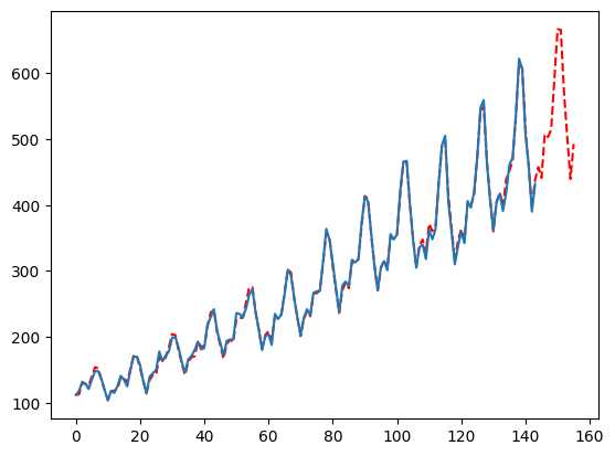
Now let’s see how to pass the config to AutoMFLES, since this is what we
use under-the-hood the results will be the same!
```python theme={null}
season_length = [12]
config = {
'seasonality_weights': [True, False],
'smoother': [True, False],
'ma': [int(min(season_length)), int(min(season_length)/2),None],
'seasonal_period': [None, season_length],
}
mfles_model = AutoMFLES(
season_length = season_length,
test_size = 12,
n_windows=2,
metric = 'smape',
config=config) # adding the config dictionary manually
mfles_model.fit(y=y)
predicted = mfles_model.predict(12)['mean']
fitted = mfles_model.predict_in_sample()['fitted']
plt.plot(np.append(fitted, predicted), linestyle='dashed', color='red')
plt.plot(y)
plt.show()
```
Let’s take a look at some of the key parameters for a standard
experience.
* **season\_length**: a list of seasonal periods, in order of perceived
importance preferably.
* **test\_size**: AutoMFLES is optimized via time series cross
validation. The test size dictates how many periods to use in each
test fold. **This is probably the most important parameter when it
comes to optimizing and you should weigh the season length, forecast
horizon, and general data length when setting this. But a good rule
of thumb is either the most important season length or half that to
allow MFLES to pick up on seasonality.**
* **n\_windows**: how many test sets are used in optimizing parameters.
In this example, 2 means that we, in total, use 24 months (12 \* 2)
split between the 2 windows.
* **metric**: this one is easy, it is simply the metric we want to
optimize for with our parameters. Here we use the default which is
smape that is defaulted to reproduce experiment results on M4. You
can also pass ‘rmse’, ‘mape’, or ‘mae’ to optimize for another
metric.
# **A deeper look at a more customized model**
The previous fit is done with 99% automated logic checks and grid
searched parameters. But we can manipulate the fit greatly (maybe too
much). This section will overview some very important parameters and how
they effect the output.
## **The parameter grid search**
First, let’s take a look at the default grid of parameters AutoMFLES
will try:
```python theme={null}
config = {
'seasonality_weights': [True, False],
'smoother': [True, False],
'ma': [int(min(seasonal_period)), int(min(seasonal_period)/2),None],
'seasonal_period': [None, seasonal_period],
}
```
* **seasonality\_weights**: If True, we will weigh more recent
observations more when calculating seasonality. The allows a
deterministic seasonality to reflect more recent changes.
* **smoother**: True means we will use a simple exponential smoother
to fit on residuals after a few rounds of boosting. If the parameter
is False then we use a simple moving average
* **ma**: This parameter is the number of past observations to include
when using a moving average, None indicates it will be semi-auto set
or disregarded in the case of ‘smoother’ being True. For optimizing
we search for the minimum season length provided by you or that
number divided by 2.
* **seasonal\_period**: this is the list of season\_length provided by
the you
Now let’s see how to pass the config to AutoMFLES, since this is what we
use under-the-hood the results will be the same!
```python theme={null}
season_length = [12]
config = {
'seasonality_weights': [True, False],
'smoother': [True, False],
'ma': [int(min(season_length)), int(min(season_length)/2),None],
'seasonal_period': [None, season_length],
}
mfles_model = AutoMFLES(
season_length = season_length,
test_size = 12,
n_windows=2,
metric = 'smape',
config=config) # adding the config dictionary manually
mfles_model.fit(y=y)
predicted = mfles_model.predict(12)['mean']
fitted = mfles_model.predict_in_sample()['fitted']
plt.plot(np.append(fitted, predicted), linestyle='dashed', color='red')
plt.plot(y)
plt.show()
```
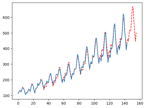
 ### What if you want to force a less reactive forecast?
Just pass False for the smoother and adjust ma to be larger relative to
your seasonality
```python theme={null}
season_length = [12]
config = {
'seasonality_weights': [True, False],
'smoother': [False],
'ma': [30],
'seasonal_period': [None, season_length],
}
mfles_model = AutoMFLES(
season_length = season_length,
test_size = 12,
n_windows=2,
metric = 'smape',
config=config) # adding the config dictionary manually
mfles_model.fit(y=y)
predicted = mfles_model.predict(12)['mean']
fitted = mfles_model.predict_in_sample()['fitted']
plt.plot(np.append(fitted, predicted), linestyle='dashed', color='red')
plt.plot(y)
plt.show()
```
### What if you want to force a less reactive forecast?
Just pass False for the smoother and adjust ma to be larger relative to
your seasonality
```python theme={null}
season_length = [12]
config = {
'seasonality_weights': [True, False],
'smoother': [False],
'ma': [30],
'seasonal_period': [None, season_length],
}
mfles_model = AutoMFLES(
season_length = season_length,
test_size = 12,
n_windows=2,
metric = 'smape',
config=config) # adding the config dictionary manually
mfles_model.fit(y=y)
predicted = mfles_model.predict(12)['mean']
fitted = mfles_model.predict_in_sample()['fitted']
plt.plot(np.append(fitted, predicted), linestyle='dashed', color='red')
plt.plot(y)
plt.show()
```
 ### **Forcing** **Seasonality**
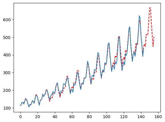
Sometimes a seasonal series is auto-fit with a nonseasonal setting, to
adjust this and force seasonality, jsut remove the ‘None’ setting in the
seasonal\_period list.
This also reduces the number of configurations MFLES tries and therefore
speeds up the fitting.
```python theme={null}
season_length = [12]
config = {
'seasonality_weights': [True, False],
'smoother': [False],
'ma': [30],
'seasonal_period': [season_length],
}
mfles_model = AutoMFLES(
season_length = season_length,
test_size = 12,
n_windows=2,
metric = 'smape',
config=config) # adding the config dictionary manually
mfles_model.fit(y=y)
predicted = mfles_model.predict(12)['mean']
fitted = mfles_model.predict_in_sample()['fitted']
plt.plot(np.append(fitted, predicted), linestyle='dashed', color='red')
plt.plot(y)
plt.show()
```
### **Forcing** **Seasonality**
Sometimes a seasonal series is auto-fit with a nonseasonal setting, to
adjust this and force seasonality, jsut remove the ‘None’ setting in the
seasonal\_period list.
This also reduces the number of configurations MFLES tries and therefore
speeds up the fitting.
```python theme={null}
season_length = [12]
config = {
'seasonality_weights': [True, False],
'smoother': [False],
'ma': [30],
'seasonal_period': [season_length],
}
mfles_model = AutoMFLES(
season_length = season_length,
test_size = 12,
n_windows=2,
metric = 'smape',
config=config) # adding the config dictionary manually
mfles_model.fit(y=y)
predicted = mfles_model.predict(12)['mean']
fitted = mfles_model.predict_in_sample()['fitted']
plt.plot(np.append(fitted, predicted), linestyle='dashed', color='red')
plt.plot(y)
plt.show()
```
 ## **Controlling the Complexity**
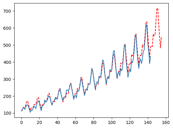
One of the best ways to control for complexity is with the max\_rounds
parameter. By default this is set to 50 but most of the time the model
converges much quicker than that. At round 4 we start implementing
smoothers as the trend piece so if you do not want that then set the
max\_rounds to 3! But, you probably want the smoothers!
```python theme={null}
season_length = [12]
config = {
'seasonality_weights': [True, False],
'smoother': [True, False],
'ma': [int(min(season_length)), int(min(season_length)/2),None],
'seasonal_period': [None, season_length],
'max_rounds': [3],
}
mfles_model = AutoMFLES(
season_length = season_length,
test_size = 12,
n_windows=2,
metric = 'smape',
config=config) # adding the config dictionary manually
mfles_model.fit(y=y)
predicted = mfles_model.predict(12)['mean']
fitted = mfles_model.predict_in_sample()['fitted']
plt.plot(np.append(fitted, predicted), linestyle='dashed', color='red')
plt.plot(y)
plt.show()
```
## **Controlling the Complexity**
One of the best ways to control for complexity is with the max\_rounds
parameter. By default this is set to 50 but most of the time the model
converges much quicker than that. At round 4 we start implementing
smoothers as the trend piece so if you do not want that then set the
max\_rounds to 3! But, you probably want the smoothers!
```python theme={null}
season_length = [12]
config = {
'seasonality_weights': [True, False],
'smoother': [True, False],
'ma': [int(min(season_length)), int(min(season_length)/2),None],
'seasonal_period': [None, season_length],
'max_rounds': [3],
}
mfles_model = AutoMFLES(
season_length = season_length,
test_size = 12,
n_windows=2,
metric = 'smape',
config=config) # adding the config dictionary manually
mfles_model.fit(y=y)
predicted = mfles_model.predict(12)['mean']
fitted = mfles_model.predict_in_sample()['fitted']
plt.plot(np.append(fitted, predicted), linestyle='dashed', color='red')
plt.plot(y)
plt.show()
```
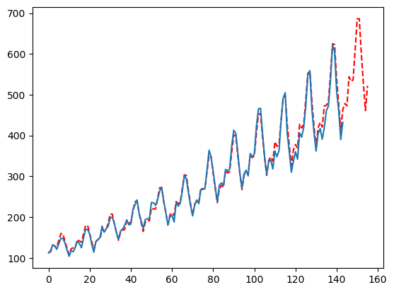
 You can also leverage estimator specific learning rates which are
applied to individual estimators rather than the entire boosting round.
Useful if you notice that the residual smoother is eating too much
signal too quickly:
```python theme={null}
season_length = [12]
config = {
'seasonality_weights': [True, False],
'smoother': [True, False],
'ma': [int(min(season_length)), int(min(season_length)/2),None],
'seasonal_period': [None, season_length],
'rs_lr': [.2],
}
mfles_model = AutoMFLES(
season_length = season_length,
test_size = 12,
n_windows=2,
metric = 'smape',
config=config) # adding the config dictionary manually
mfles_model.fit(y=y)
predicted = mfles_model.predict(12)['mean']
fitted = mfles_model.predict_in_sample()['fitted']
plt.plot(np.append(fitted, predicted), linestyle='dashed', color='red')
plt.plot(y)
plt.show()
```
You can also leverage estimator specific learning rates which are
applied to individual estimators rather than the entire boosting round.
Useful if you notice that the residual smoother is eating too much
signal too quickly:
```python theme={null}
season_length = [12]
config = {
'seasonality_weights': [True, False],
'smoother': [True, False],
'ma': [int(min(season_length)), int(min(season_length)/2),None],
'seasonal_period': [None, season_length],
'rs_lr': [.2],
}
mfles_model = AutoMFLES(
season_length = season_length,
test_size = 12,
n_windows=2,
metric = 'smape',
config=config) # adding the config dictionary manually
mfles_model.fit(y=y)
predicted = mfles_model.predict(12)['mean']
fitted = mfles_model.predict_in_sample()['fitted']
plt.plot(np.append(fitted, predicted), linestyle='dashed', color='red')
plt.plot(y)
plt.show()
```
 ## **Tips and Tricks**
Since most settings are optimized for during cross validation there is
always a trade-off between accuracy and computation.
The default settings were done after extensive testing to give you a
balanced approach. Hopefully, it delivers good accuracy in a short
amount of time.
But, there are ways to give you generally more accuracy (not life
changing but a slight boost) or a dramatic decrease in runtime (without
sacrificing too much accuracy).
The next section will review some of those settings!
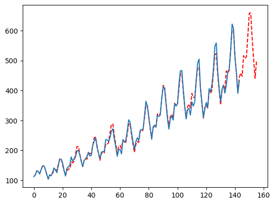
## **Number of Testing Windows**
When optimizing using time series cross validation the number of windows
directly effects the number of times we have to fit the model for each
parameter. The default here is 2, but going up to 3 (if your data allows
it) should give you more consistent results. Obviously, the more the
better to a certain point but this will depend on your data. Conversely,
decreasing this to 1 means you are choosing parameters based on a single
holdout set which may decrease accuracy.
```python theme={null}
season_length = [12]
mfles_model = AutoMFLES(
season_length = season_length,
test_size = 12,
n_windows = 1, # Trying just 1 window here
metric = 'smape')
mfles_model.fit(y=y)
predicted = mfles_model.predict(12)['mean']
fitted = mfles_model.predict_in_sample()['fitted']
plt.plot(np.append(fitted, predicted), linestyle='dashed', color='red')
plt.plot(y)
plt.show()
```
## **Tips and Tricks**
Since most settings are optimized for during cross validation there is
always a trade-off between accuracy and computation.
The default settings were done after extensive testing to give you a
balanced approach. Hopefully, it delivers good accuracy in a short
amount of time.
But, there are ways to give you generally more accuracy (not life
changing but a slight boost) or a dramatic decrease in runtime (without
sacrificing too much accuracy).
The next section will review some of those settings!
## **Number of Testing Windows**
When optimizing using time series cross validation the number of windows
directly effects the number of times we have to fit the model for each
parameter. The default here is 2, but going up to 3 (if your data allows
it) should give you more consistent results. Obviously, the more the
better to a certain point but this will depend on your data. Conversely,
decreasing this to 1 means you are choosing parameters based on a single
holdout set which may decrease accuracy.
```python theme={null}
season_length = [12]
mfles_model = AutoMFLES(
season_length = season_length,
test_size = 12,
n_windows = 1, # Trying just 1 window here
metric = 'smape')
mfles_model.fit(y=y)
predicted = mfles_model.predict(12)['mean']
fitted = mfles_model.predict_in_sample()['fitted']
plt.plot(np.append(fitted, predicted), linestyle='dashed', color='red')
plt.plot(y)
plt.show()
```
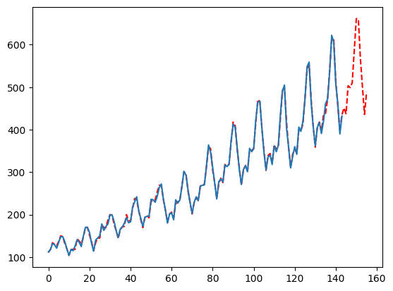
 And now trying with 3, notice the fit is different!
```python theme={null}
season_length = [12]
mfles_model = AutoMFLES(
season_length = season_length,
test_size = 12,
n_windows = 3, # Trying just 1 window here
metric = 'smape')
mfles_model.fit(y=y)
predicted = mfles_model.predict(12)['mean']
fitted = mfles_model.predict_in_sample()['fitted']
plt.plot(np.append(fitted, predicted), linestyle='dashed', color='red')
plt.plot(y)
plt.show()
```
And now trying with 3, notice the fit is different!
```python theme={null}
season_length = [12]
mfles_model = AutoMFLES(
season_length = season_length,
test_size = 12,
n_windows = 3, # Trying just 1 window here
metric = 'smape')
mfles_model.fit(y=y)
predicted = mfles_model.predict(12)['mean']
fitted = mfles_model.predict_in_sample()['fitted']
plt.plot(np.append(fitted, predicted), linestyle='dashed', color='red')
plt.plot(y)
plt.show()
```
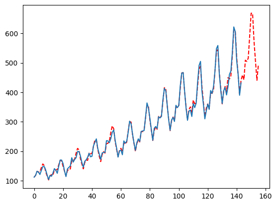
 ## **The Moving Average Parameter**
By default, we will try the min of your season lengths and half that for
the ‘ma’ parameter. This works well in the wild but you may want to
deepen this search greatly. **This is one of the best parameters to
tweak if you need more accuracy out of MFLES**. Simply pass more
parameters to the list, ideally these numbers are informed by the
seasonality, forecast horizon, or some other bit of information. In our
case, I will also pass 3 and 4 due to it being monthly data. Since this
increases the number of parameters to try, it will also increase the
computation time.
```python theme={null}
season_length = [12]
config = {
'seasonality_weights': [True, False],
'smoother': [True, False],
'ma': [3, 4, int(min(season_length)), int(min(season_length)/2),None],
'seasonal_period': [None, season_length],
}
mfles_model = AutoMFLES(
season_length = season_length,
test_size = 12,
n_windows=2,
metric = 'smape',
config=config) # adding the config dictionary manually
mfles_model.fit(y=y)
predicted = mfles_model.predict(12)['mean']
fitted = mfles_model.predict_in_sample()['fitted']
plt.plot(np.append(fitted, predicted), linestyle='dashed', color='red')
plt.plot(y)
plt.show()
```
## **The Moving Average Parameter**
By default, we will try the min of your season lengths and half that for
the ‘ma’ parameter. This works well in the wild but you may want to
deepen this search greatly. **This is one of the best parameters to
tweak if you need more accuracy out of MFLES**. Simply pass more
parameters to the list, ideally these numbers are informed by the
seasonality, forecast horizon, or some other bit of information. In our
case, I will also pass 3 and 4 due to it being monthly data. Since this
increases the number of parameters to try, it will also increase the
computation time.
```python theme={null}
season_length = [12]
config = {
'seasonality_weights': [True, False],
'smoother': [True, False],
'ma': [3, 4, int(min(season_length)), int(min(season_length)/2),None],
'seasonal_period': [None, season_length],
}
mfles_model = AutoMFLES(
season_length = season_length,
test_size = 12,
n_windows=2,
metric = 'smape',
config=config) # adding the config dictionary manually
mfles_model.fit(y=y)
predicted = mfles_model.predict(12)['mean']
fitted = mfles_model.predict_in_sample()['fitted']
plt.plot(np.append(fitted, predicted), linestyle='dashed', color='red')
plt.plot(y)
plt.show()
```
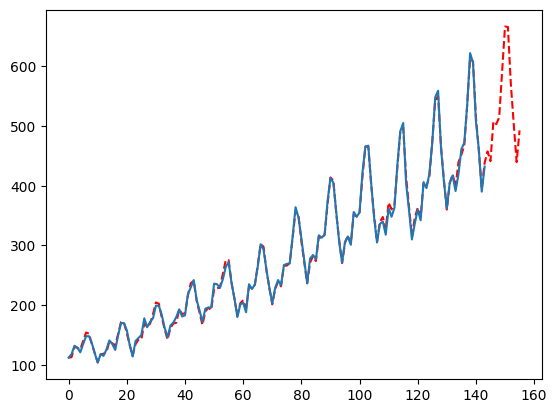
 ### **Changepoints**
By default, MFLES will auto-detect if it should use changepoints. This
has some accuracy benefits but massive computation expenses. You can
disable changepoints and generally see close accuracy but great speed
gains:
```python theme={null}
season_length = [12]
config = {
'changepoints': [False],
'seasonality_weights': [True, False],
'smoother': [True, False],
'ma': [int(min(season_length)), int(min(season_length)/2),None],
'seasonal_period': [None, season_length],
}
mfles_model = AutoMFLES(
season_length = season_length,
test_size = 12,
n_windows=2,
metric = 'smape',
config=config) # adding the config dictionary manually
mfles_model.fit(y=y)
predicted = mfles_model.predict(12)['mean']
fitted = mfles_model.predict_in_sample()['fitted']
plt.plot(np.append(fitted, predicted), linestyle='dashed', color='red')
plt.plot(y)
plt.show()
```
### **Changepoints**
By default, MFLES will auto-detect if it should use changepoints. This
has some accuracy benefits but massive computation expenses. You can
disable changepoints and generally see close accuracy but great speed
gains:
```python theme={null}
season_length = [12]
config = {
'changepoints': [False],
'seasonality_weights': [True, False],
'smoother': [True, False],
'ma': [int(min(season_length)), int(min(season_length)/2),None],
'seasonal_period': [None, season_length],
}
mfles_model = AutoMFLES(
season_length = season_length,
test_size = 12,
n_windows=2,
metric = 'smape',
config=config) # adding the config dictionary manually
mfles_model.fit(y=y)
predicted = mfles_model.predict(12)['mean']
fitted = mfles_model.predict_in_sample()['fitted']
plt.plot(np.append(fitted, predicted), linestyle='dashed', color='red')
plt.plot(y)
plt.show()
```
 ### **Seasonality Weights**
Most time series will not have a significant shift in the seasonal
signal, or at least not one that is worth the extra computation needed
to fit for it. To speed things up a bit, you can disable this. Although,
sometimes, disabling this will cause large degradation in accuracy.
```python theme={null}
season_length = [12]
config = {
'seasonality_weights': [False],
'smoother': [True, False],
'ma': [int(min(season_length)), int(min(season_length)/2),None],
'seasonal_period': [None, season_length],
}
mfles_model = AutoMFLES(
season_length = season_length,
test_size = 12,
n_windows=2,
metric = 'smape',
config=config) # adding the config dictionary manually
mfles_model.fit(y=y)
predicted = mfles_model.predict(12)['mean']
fitted = mfles_model.predict_in_sample()['fitted']
plt.plot(np.append(fitted, predicted), linestyle='dashed', color='red')
plt.plot(y)
plt.show()
```
### **Seasonality Weights**
Most time series will not have a significant shift in the seasonal
signal, or at least not one that is worth the extra computation needed
to fit for it. To speed things up a bit, you can disable this. Although,
sometimes, disabling this will cause large degradation in accuracy.
```python theme={null}
season_length = [12]
config = {
'seasonality_weights': [False],
'smoother': [True, False],
'ma': [int(min(season_length)), int(min(season_length)/2),None],
'seasonal_period': [None, season_length],
}
mfles_model = AutoMFLES(
season_length = season_length,
test_size = 12,
n_windows=2,
metric = 'smape',
config=config) # adding the config dictionary manually
mfles_model.fit(y=y)
predicted = mfles_model.predict(12)['mean']
fitted = mfles_model.predict_in_sample()['fitted']
plt.plot(np.append(fitted, predicted), linestyle='dashed', color='red')
plt.plot(y)
plt.show()
```