> ## Documentation Index
> Fetch the complete documentation index at: https://nixtlaverse.nixtla.io/llms.txt
> Use this file to discover all available pages before exploring further.
# AutoRegressive Model
> Step-by-step guide on using the `AutoRegressive Model` with
> `Statsforecast`.
During this walkthrough, we will become familiar with the main
`StatsForecast` class and some relevant methods such as
`StatsForecast.plot`, `StatsForecast.forecast` and
`StatsForecast.cross_validation` in other.
The text in this article is largely taken from: 1. [Changquan Huang •
Alla Petukhina. Springer series (2022). Applied Time Series Analysis and
Forecasting with
Python.](https://link.springer.com/book/10.1007/978-3-031-13584-2) 2.
[Jose A. Fiorucci, Tiago R. Pellegrini, Francisco Louzada, Fotios
Petropoulos, Anne B. Koehler (2016). “Models for optimising the theta
method and their relationship to state space models”. International
Journal of
Forecasting](https://www.sciencedirect.com/science/article/pii/S0169207016300243).
3\. [Rob J. Hyndman and George Athanasopoulos (2018). “Forecasting
Principles and Practice (3rd ed)”](https://otexts.com/fpp3/tscv.html)
## Table of Contents
* [Introduction](#introduction)
* [Autoregressive Models](#model)
* [Loading libraries and data](#loading)
* [Explore data with the plot method](#plotting)
* [Split the data into training and testing](#splitting)
* [Implementation of AutoRegressive with
StatsForecast](#implementation)
* [Cross-validation](#cross_validate)
* [Model evaluation](#evaluate)
* [References](#references)
## Introduction
The `autoregressive` time series model `(AutoRegressive)` is a
`statistical` technique used to analyze and predict univariate time
series. In essence, the `autoregressive model` is based on the idea that
previous values of the time series can be used to predict future values.
In this model, the dependent variable (the time series) returns to
itself at different moments in time, creating a dependency relationship
between past and present values. The idea is that past values can help
us understand and predict future values of the series.
The `autoregressive model` can be fitted to different orders, which
indicate how many past values are used to predict the present value. For
example, an `autoregressive model` of order 1 $(AR(1))$ uses only the
immediately previous value to predict the current value, while an
`autoregressive model` of order $p (AR(p))$ uses the $p$ previous
values.
The `autoregressive model` is one of the basic models of time series
analysis and is widely used in a variety of fields, from finance and
economics to meteorology and social sciences. The model’s ability to
capture nonlinear dependencies in time series data makes it especially
useful for forecasting and long-term trend analysis.
In a `multiple regression model`, we forecast the variable of interest
using a linear combination of predictors. In an `autoregression model`,
we forecast the variable of interest using a `linear combination` of
past values of the variable. The term `autoregression` indicates that it
is a regression of the variable against itself.
## Definition of Autoregressive Models
Before giving a formal definition of the ARCH model, let’s define the
components of an ARCH model in a general way:
* Autoregressive, a concept that we have already known, is the
construction of a univariate time series model using statistical
methods, which means that the current value of a variable is
influenced by past values of itself in different periods.
* Heteroscedasticity means that the model can have different
magnitudes or variability at different time points (variance changes
over time).
* Conditional, since volatility is not fixed, the reference here is
the constant that we put in the model to limit heteroscedasticity
and make it conditionally dependent on the previous value or values
of the variable.
The AR model is the most basic building block of univariate time series.
As you have seen before, univariate time series are a family of models
that use only information about the target variable’s past to forecast
its future, and do not rely on other explanatory variables.
**Definition 1.** (1) The following equation is called the
autoregressive model of order $p$ and denoted by $\text{AR(p)}$:
$$
\begin{equation}
Xt =\varphi_0 +\varphi_1X_{t−1}+\varphi_2X_{t−2}+\cdots+\varphi_p X_{t−p}+\varepsilon_t \tag 1
\end{equation}
$$
where $\{\varepsilon_t \} \sim WN(0,\sigma_{\epsilon}^2)$,
$E(X_s \varepsilon_t) = 0$ if $s < t$ and
$\varphi_0,\varphi_1,\cdots ,\varphi_p$ are real-valued parameters
(coefficients) with $\varphi_p \neq 0$.
1. If a time series $\{X_t \}$ is stationary and satisfies such an
equation as (1), then we call it an $\text{AR(p)}$ process.
Note the following remarks about this definition:
* For simplicity, we often assume that the intercept (const term)
$\varphi_0 = 0$; otherwise, we can consider $\{X_t −\mu \}$ where
$\mu =\varphi_0 /(1−\varphi_1 − \cdots −\varphi_p)$.
* We distinguish the concept of $\text{AR}$ models from the concept of
$\text{AR}$ processes. $\text{AR}$ models may or may not be
stationary and $\text{AR}$ processes must be stationary.
* $E(X_s \varepsilon_t) = 0(s < t)$ means that $X_s$ in the past has
nothing to do with $\varepsilon_t$ at the current time $t$.
* Like the definition of MA models, sometimes εt in Eq.(1) is called
the innovation or shock term.
In addition, using the
backshift([see](https://otexts.com/fpp3/backshift.html)) operator $B$,
the $\text{AR(p)}$ model can be rewritten as
$\varphi(B)X_t = \varepsilon_t$
where $\varphi(z) = 1 − \varphi_1z − \cdots − \varphi_p z^p$ is called
the (corresponding) $\text{AR}$ polynomial. Besides, in the Python
package |StatsModels|, $\varphi(B)$ is called the $\text{AR}$ lag
polynomial.
### Definition of PACF
Let $\{X_t \}$ be a stationary time series with $E(X_t) = 0$. Here the
assumption $E(X_t ) = 0$ is for conciseness only. If
$E(X_t) = \mu \neq 0$, it is okay to replace $\{X_t \}$ by
$\{X_t − \mu \}$. Now consider the linear regression (prediction) of
$X_t$ on $\{X_{t−k+1:t−1} \}$ for any integer $k ≥ 2$. We use $\hat X_t$
to denote this regression (prediction):
$\hat X_t =\alpha_1 X_{t−1}+ \cdots +\alpha_{k−1} X_{t−k+1}$
where $\{\alpha_1, \cdots , \alpha_{k−1} \}$ satisfy
$\{\alpha_1, \cdots , \alpha_{k−1} \}=\argmin_{β1,···,βk−1} E[X_t −(\beta_1 X_{t−1} +\cdots +\beta_{k−1}X_{t−k+1})]^2$
That is, $\{\alpha_1, \cdots , \alpha_{k−1} \}$ are chosen by minimizing
the mean squared error of prediction. Similarly, let $\hat X_{t −k}$
denote the regression (prediction) of $X_{t −k}$ on
$\{X_{t −k+1:t −1} \}$:
$\hat X_{t−k} =\eta_1 X_{t−1}+ \cdots +\eta_{k−1} X_{t−k+1}$
Note that if $\{X_t \}$ is stationary, then
$\{ \alpha_{1:k−1}\} = \{\eta_{1:k−1} \}$. Now let
$\hat Z_{t−k} = X_{t−k} − \hat X_{t−k}$ and $\hat Z_t = X_t − \hat X_t$.
Then $\hat Z_{t−k}$ is the residual of removing the effect of the
intervening variables $\{X_{t−k+1:t−1} \}$ from $X_{t−k}$, and
$\hat Z_t$ is the residual of removing the effect of
$\{X_{t −k+1:t −1} \}$ from $X_t$.
**Definition 2.** The partial autocorrelation function(PACF) at lag $k$
of astationary time series $\{X_t \}$ with $E(X_t ) = 0$ is
$\phi_{11} = Corr(X_{t−1}, X_t ) = \frac{Cov(X_{t−1}, X_t )} {[Var(X_{t−1})Var(X_t)]^1/2}=\rho_1$
and
$\phi_{kk} = Corr(\hat Z_{t−k},\hat Z_t)=\frac{Cov(\hat Z_{t−k},\hat Z_t)} {[Var(\hat Z_{t−k})Var(\hat Z_t)]^{1/2}}$
According to the property of correlation coefficient (see, e.g., P172,
Casella and Berger 2002), |φkk| ≤ 1. On the other hand, the following
theorem paves the way to estimate the PACF of a stationary time series,
and its proof can be seen in Fan and Yao (2003).
On the other hand, the following theorem paves the way to estimate the
PACF of a stationary time series, and its proof can be seen in Fan and
Yao (2003).
**Theorem 1.** Let $\{X_t \}$ be a stationary time series with
$E(X_t) = 0$, and $\{a_{1k},\cdots ,a_{kk} \}$ satisfy
$\{a_{1k},\cdots,a_{kk} \}=\argmin_{a_1 ,\cdots ,a_k} E(X_{t −a1}X_{t−1}−\cdots −a_k X_{t−k})^2$
Then $\phi_{kk}=a_{kk}$ for $k≥1$.
### Properties of Autoregressive Models
From the $\text{AR(p)}$ model, namely, Eq. (1), we can see that it is in
the same form as the multiple linear regression model. However, it
explains current itself with its own past. Given the past
$\{X_{(t−p):(t−1)} \} = \{x_{(t−p):(t−1)} \}$
we have
$E(X_t |X_{(t−p):(t−1)}) = \varphi_0 + \varphi_1x_{t−1} + \varphi_2 x_{t−2} + \cdots + \varphi_p x_{t−p}$
This suggests that given the past, the right-hand side of this equation
is a good estimate of $X_t$ . Besides
$Var(X_t |X_{(t −p):(t −1)}) = Var(\varepsilon_t ) = \sigma_{\varepsilon}^2$
Now we suppose that the AR(p) model, namely, Eq. (1), is stationary;
then we have
1. The model mean $E(_Xt)=\mu =\varphi_0 / (1−\varphi_1−···−\varphi_p)$
.Thus,themodelmean $\mu=0$ if and only if $\varphi_0 =0$.
2. If the mean is zero or $\varphi_0 = 0$ ((3) and (4) below have the
same assumption), noting that
$E(X_t \varepsilon_t ) = \sigma_{\varepsilon}^2$ , we multiply
Eq. (1) by $X_t$ , take expectations, and then get
$\text {Var} (X_t) = \gamma_0 = \varphi_1 \gamma_1 + \varphi_2 \gamma2 + \cdots + \varphi_p \gamma_p + \sigma_{\varepsilon}^2$
Furthermore
$\gamma_0 = \sigma_{\varepsilon}^2 / ( 1 − \varphi_1 \rho_1 − \varphi_2 \rho_2 − \cdots − \varphi_p \rho_p )$
1. For all $k > p$, the partial autocorrelation $\phi_{kk} = 0$, that
is, the PACF of $\text{AR(p)}$ models cuts off after lag $p$, which
is very helpful in identifying an $\text{AR}$ model. In fact, at
this point, the predictor or regression of $X_t$ on
$\{X_{t−k+1:t−1} \}$ is
$\hat X_t =\varphi_1 X_{t−1}+\cdots +\varphi_{k−1} X_{t−k+1}$
Thus, $X_t − \hat X_t = \varepsilon_t$. Moreover,
$X_{t−k} − \hat X_{t−k}$ is a function of $\{ X_{t−k:t−1} \}$, and
$\varepsilon_t$ is uncorrelated to everyone in $\{X_{t−k:t−1} \}$.
Therefore
$Cov(X_{t−k} −\hat X_{t−k},X_t −\hat X_t)=Cov(X_{t−k} −\hat X_{t−k},\varepsilon_t)=0.$
By Definition 2, $\phi_{kk} = 0$.
1. We multiply Eq.(1)by $X_{t−k}$,take expectations,divide by
$\gamma_0$,and then obtain the recursive relationship between the
autocorrelations:
$$
\begin{equation}
for \ k ≥ 1, \rho_k = \varphi_1 \rho_{k−1} + \varphi_2 \rho_{k−2} + \cdots + \varphi_p \rho_{k−p} \tag 2
\end{equation}
$$
For Eq.(2), let $k = 1,2,··· ,p$. Then we arrive at a set of difference
equations, which is known as the Yule-Walker equations. If the
$\text{ACF} \{\rho_{1:p} \}$ are given, then we can solve the
Yule-Walker equations to obtain the estimates for $\{\varphi_{1:p} \}$,
and the solutions are called the Yule-Walker estimates.
1. Since the model is a stationary $\text{AR(p)}$ now, naturally it
satisfies
$X_t =\varphi_1 X_{t−1}+ \varphi_2 X_{t−2} + \cdots + \varphi_p X_{t−p} + \varepsilon_t$.
Hence $\phi_{pp} = \varphi_p$. If the $\text{AR(p)}$ model is
further Gaussian and a sample of size $\text{T}$ is given, then (a)
$\hat \phi_{pp} → \varphi_p$ as $T → ∞$; (b) according to Quenouille
(1949), for $k > p, \sqrt{T} \hat \phi_{kk}$ asymptotically follows
the standard normal(Gaussian) distribution $\text{N(0,1)}$, or
$\phi_{kk}$ is asymptotically distributed as $\text{N(0, 1/T )}$.
### Stationarity and Causality of AR Models
Consider the AR(1) model:
$$
\begin{equation}
X_t = \varphi X_{t − 1} + \varepsilon_t , \varepsilon_t \sim W N( 0 , \sigma_{\varepsilon}^2 ) \tag 3
\end{equation}
$$
For $|\varphi|<1$,let
$X_{1t} =\sum_{j=0}^{\infty} \varphi^j \varepsilon_{t−j}$ and for
$|\varphi|>1$,let
$X_{2t} =− \sum_{j=1}^{\infty} \varphi^{-j} \varepsilon_{t+j}$. It is
easy to show that both $\{X_{1t } \}$ and $\{X_{2t } \}$ are stationary
and satisfy Eq. (3). That is, both are the stationary solution of Eq.
(3). This gives rise to a question: which one of both is preferable?
Obviously, $\{X_{2t } \}$ depends on future values of unobservable
$\{\varepsilon_t \}$, and so it is unnatural. Hence we take
$\{X_{1t } \}$ and abandon $\{X_{2t } \}$. In other words, we require
that the coefficient $\varphi$ in Eq. (3) is less 1 in absolute value.
At this point, the $\text{AR}(1)$ model is said to be causal and its
causal expression is
$X_t = \sum_{j=0}^{\infty} \varphi^j \varepsilon_{t−j}$. In general, the
definition of causality is given below.
**Definition 3** (1) A time series $\{X_t \}$ is causal if there exist
coefficients $\psi_j$ such that
$X_t =\sum_{j=0}^{\infty} \psi_j \varepsilon_{t-j}, \ \ \sum_{j=0}^{\infty} |\psi_j |< \infty$
where
$\psi_0 = 1, \{\varepsilon_t \} \sim WN(0, \sigma_{\varepsilon}^2 )$. At
this point, we say that the time series $\{X_t \}$ has an
$\text{MA}(\infty)$ representation.
1. We say that a model is causal if the time series generated by it is
causal.
Causality suggests that the time series $\{X_t\}$ is caused by the white
noise (or innovations) from the past up to time t . Besides, the time
series $\{X_{2t } \}$ is an example that is stationary but not causal.
In order to determine whether an $\text{AR}$ model is causal, similar to
the invertibility for the $\text{MA}$ model, we have the following
theorem.
**Theorem 2(CausalityTheorem)** An $\text{AR}$ model defined by Eq.(1)
is causal if and only if the roots of its $\text{AR}$ polynomial
$\varphi(z)=1−\varphi_1 z− \cdots − \varphi_p z^p$ exceed 1 in modulus
or lie outside the unit circle on the complex plane.
Note the following remarks: \* In the light of the existence and
uniqueness on page 75 of Brockwell and Davis (2016), an $\text{AR}$
model defined by Eq.(1) is stationary if and only if its $\text{AR}$
polynomial $\varphi(z)=1−\varphi_1 z− \cdots − \varphi_p z^p \neq 0$ for
all $|z|=1$ or all the roots of the $\text{AR}$ polynomial do not lie on
the unit circle. Hence for the AR model defined by Eq. (1), its
stationarity condition is weaker than its causality condition.
* A causal time series is surely a stationary one. So an $\text{AR}$
model that satisfies the causal condition is naturally stationary.
But a stationary $\text{AR}$ model is not necessarily causal.
* If the time series $\{X_t \}$ generated by Eq. (1) is not from the
remote past, namely,
$t \in T = {\cdots ,−n,\cdots ,−1,0,1,\cdots ,n,\cdots}$
but starts from an initial value $X_0$, then it may be nonstationary,
not to mention causality.
* According to the relationship between the roots and the coefficients
of the degree 2 polynomial
$\varphi(z) = 1 − \varphi_1 z − \varphi_2 z^2$, it may be proved
that both of the roots of the polynomial exceed 1 in modulus if and
only if
Thus, we can conveniently use the three inequations to decide whether a
$\text{AR(2)}$ model is causal or not.
* It may be shown that for an $\text{AR(p)}$ model defined by Eq. (1),
the coefficients $\{\psi_j \}$ in Definition 3 satisfy $\psi_0=1$
and
$\psi_j=\sum_{k=1}^{j} \varphi '_k \psi_{j-k}, \ \ j \geq 1 \ where \ \ \varphi '_k =\varphi_k \ \ if \ \ k \leq p \ \ and \ \ \varphi '_k =0 \ \ if \ \ k>p$
### Autocorrelation: the past influences the present
The autoregressive model describes a relationship between the present of
a variable and its past. Therefore, it is suitable for variables in
which the past and present values are correlated.
As an intuitive example, consider the waiting line at the doctor.
Imagine that the doctor has a plan in which each patient has 20 minutes
with him. If each patient takes exactly 20 minutes, this works well. But
what if a patient takes a little longer? An autocorrelation could be
present if the duration of one query has an impact on the duration of
the next query. So if the doctor needs to speed up an appointment
because the previous appointment took too long, look at a correlation
between the past and the present. Past values influence future values.
### Positive and negative autocorrelation
Like “regular” correlation, autocorrelation can be positive or negative.
Positive autocorrelation means that a high value now is likely to give a
high value in the next period. This can be observed, for example, in
stock trading: as soon as a lot of people want to buy a stock, its price
goes up. This positive trend makes people want to buy this stock even
more as it has positive returns. The more people buy the stock, the
higher it goes and the more people will want to buy it.
A positive correlation also works in downtrends. If today’s stock value
is low, tomorrow’s value is likely to be even lower as people start
selling. When many people sell, the value falls, and even more people
will want to sell. This is also a case of positive autocorrelation since
the past and the present go in the same direction. If the past is low,
the present is low; and if the past is high, the present is high.
There is negative autocorrelation if two trends are opposite. This is
the case in the example of the duration of the doctor’s visit. If one
query takes longer, the next one will be shorter. If one visit takes
less time, the doctor may take a little longer for the next one.
### Stationarity and the ADF test
The problem of having a trend in our data is general in univariate time
series modeling. The stationarity of a time series means that a time
series does not have a (long-term) trend: it is stable around the same
average. Otherwise, a time series is said to be non-stationary.
In theory, AR models can have a trend coefficient in the model, but
since stationarity is an important concept in general time series
theory, it’s best to learn to deal with it right away. Many models can
only work on stationary time series.
A time series that is growing or falling strongly over time is obvious
to spot. But sometimes it’s hard to tell if a time series is stationary.
This is where the Augmented Dickey Fuller (ADF) test comes in handy.
## Loading libraries and data
> **Tip**
>
> Statsforecast will be needed. To install, see
> [instructions](../getting-started/installation.html).
Next, we import plotting libraries and configure the plotting style.
```python theme={null}
import pandas as pd
import scipy.stats as stats
import statsmodels.api as sm
import statsmodels.tsa.api as smt
```
```python theme={null}
import matplotlib.pyplot as plt
import seaborn as sns
from statsmodels.graphics.tsaplots import plot_acf, plot_pacf
plt.style.use('fivethirtyeight')
plt.rcParams['lines.linewidth'] = 1.5
dark_style = {
'figure.facecolor': '#212946',
'axes.facecolor': '#212946',
'savefig.facecolor':'#212946',
'axes.grid': True,
'axes.grid.which': 'both',
'axes.spines.left': False,
'axes.spines.right': False,
'axes.spines.top': False,
'axes.spines.bottom': False,
'grid.color': '#2A3459',
'grid.linewidth': '1',
'text.color': '0.9',
'axes.labelcolor': '0.9',
'xtick.color': '0.9',
'ytick.color': '0.9',
'font.size': 12 }
plt.rcParams.update(dark_style)
from pylab import rcParams
rcParams['figure.figsize'] = (18,7)
```
### Read Data
```python theme={null}
df= pd.read_csv("https://raw.githubusercontent.com/Naren8520/Serie-de-tiempo-con-Machine-Learning/main/Data/catfish.csv")
df.head()
```
| | Date | Total |
| - | --------- | ----- |
| 0 | 1986-1-01 | 9034 |
| 1 | 1986-2-01 | 9596 |
| 2 | 1986-3-01 | 10558 |
| 3 | 1986-4-01 | 9002 |
| 4 | 1986-5-01 | 9239 |
The input to StatsForecast is always a data frame in long format with
three columns: unique\_id, ds and y:
* The `unique_id` (string, int or category) represents an identifier
for the series.
* The `ds` (datestamp) column should be of a format expected by
Pandas, ideally YYYY-MM-DD for a date or YYYY-MM-DD HH:MM:SS for a
timestamp.
* The `y` (numeric) represents the measurement we wish to forecast.
```python theme={null}
df["unique_id"]="1"
df.columns=["ds", "y", "unique_id"]
df.head()
```
| | ds | y | unique\_id |
| - | --------- | ----- | ---------- |
| 0 | 1986-1-01 | 9034 | 1 |
| 1 | 1986-2-01 | 9596 | 1 |
| 2 | 1986-3-01 | 10558 | 1 |
| 3 | 1986-4-01 | 9002 | 1 |
| 4 | 1986-5-01 | 9239 | 1 |
```python theme={null}
print(df.dtypes)
```
```text theme={null}
ds object
y int64
unique_id object
dtype: object
```
We can see that our time variable `ds` is in an object format, we need
to convert to a date format
```python theme={null}
df["ds"] = pd.to_datetime(df["ds"])
```
## Explore data with the plot method
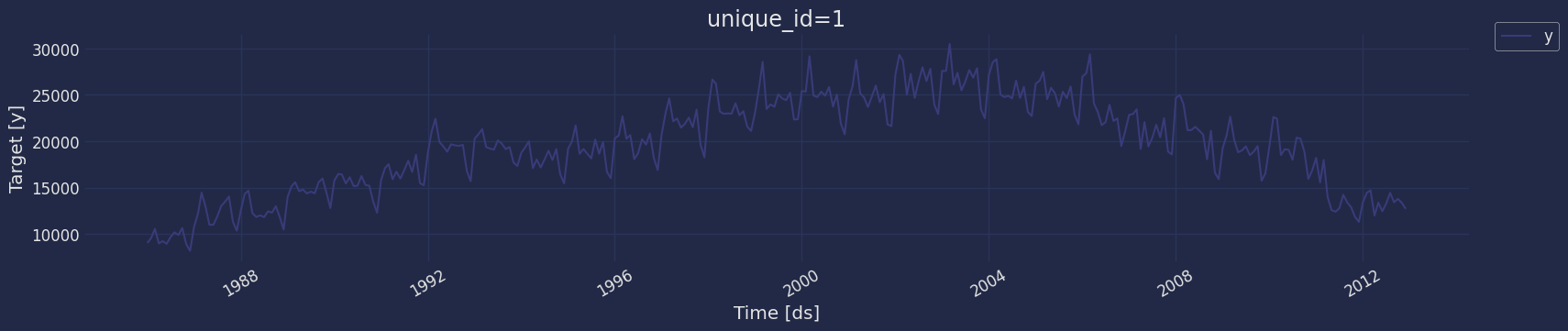
Plot some series using the plot method from the StatsForecast class.
This method prints 8 random series from the dataset and is useful for
basic EDA.
```python theme={null}
from statsforecast import StatsForecast
StatsForecast.plot(df)
```
 ### The Augmented Dickey-Fuller Test
An Augmented Dickey-Fuller (ADF) test is a type of statistical test that
determines whether a unit root is present in time series data. Unit
roots can cause unpredictable results in time series analysis. A null
hypothesis is formed in the unit root test to determine how strongly
time series data is affected by a trend. By accepting the null
hypothesis, we accept the evidence that the time series data is not
stationary. By rejecting the null hypothesis or accepting the
alternative hypothesis, we accept the evidence that the time series data
is generated by a stationary process. This process is also known as
stationary trend. The values of the ADF test statistic are negative.
Lower ADF values indicate a stronger rejection of the null hypothesis.
Augmented Dickey-Fuller Test is a common statistical test used to test
whether a given time series is stationary or not. We can achieve this by
defining the null and alternate hypothesis.
Null Hypothesis: Time Series is non-stationary. It gives a
time-dependent trend. Alternate Hypothesis: Time Series is stationary.
In another term, the series doesn’t depend on time.
ADF or t Statistic \< critical values: Reject the null hypothesis, time
series is stationary. ADF or t Statistic > critical values: Failed to
reject the null hypothesis, time series is non-stationary.
Let’s check if our series that we are analyzing is a stationary series.
Let’s create a function to check, using the `Dickey Fuller` test
```python theme={null}
from statsmodels.tsa.stattools import adfuller
```
```python theme={null}
def Augmented_Dickey_Fuller_Test_func(series , column_name):
print (f'Dickey-Fuller test results for columns: {column_name}')
dftest = adfuller(series, autolag='AIC')
dfoutput = pd.Series(dftest[0:4], index=['Test Statistic','p-value','No Lags Used','Number of observations used'])
for key,value in dftest[4].items():
dfoutput['Critical Value (%s)'%key] = value
print (dfoutput)
if dftest[1] <= 0.05:
print("Conclusion:====>")
print("Reject the null hypothesis")
print("The data is stationary")
else:
print("Conclusion:====>")
print("The null hypothesis cannot be rejected")
print("The data is not stationary")
```
```python theme={null}
Augmented_Dickey_Fuller_Test_func(df["y"],'Sales')
```
```text theme={null}
Dickey-Fuller test results for columns: Sales
Test Statistic -1.589903
p-value 0.488664
No Lags Used 14.000000
...
Critical Value (1%) -3.451691
Critical Value (5%) -2.870939
Critical Value (10%) -2.571778
Length: 7, dtype: float64
Conclusion:====>
The null hypothesis cannot be rejected
The data is not stationary
```
In the previous result we can see that the `Augmented_Dickey_Fuller`
test gives us a `p-value` of 0.488664, which tells us that the null
hypothesis cannot be rejected, and on the other hand the data of our
series are not stationary.
We need to differentiate our time series, in order to convert the data
to stationary.
```python theme={null}
Augmented_Dickey_Fuller_Test_func(df["y"].diff().dropna(),"Sales")
```
```text theme={null}
Dickey-Fuller test results for columns: Sales
Test Statistic -4.310935
p-value 0.000425
No Lags Used 17.000000
...
Critical Value (1%) -3.451974
Critical Value (5%) -2.871063
Critical Value (10%) -2.571844
Length: 7, dtype: float64
Conclusion:====>
Reject the null hypothesis
The data is stationary
```
By applying a differential, our time series now is stationary.
```python theme={null}
def tsplot(y, lags=None, figsize=(12, 7), style='bmh'): # [3]
if not isinstance(y, pd.Series):
y = pd.Series(y)
with plt.style.context(style):
fig = plt.figure(figsize=figsize)
layout = (2, 2)
ts_ax = plt.subplot2grid(layout, (0, 0), colspan=2)
acf_ax = plt.subplot2grid(layout, (1, 0))
pacf_ax = plt.subplot2grid(layout, (1, 1))
y.plot(ax=ts_ax)
p_value = sm.tsa.stattools.adfuller(y)[1]
ts_ax.set_title('Time Series Analysis plot\n Dickey-Fuller: p={0:.5f}'.format(p_value))
smt.graphics.plot_acf(y, lags=lags, ax=acf_ax)
smt.graphics.plot_pacf(y, lags=lags, ax=pacf_ax)
plt.tight_layout()
```
```python theme={null}
tsplot(df["y"].diff().dropna(), lags=20);
```
### The Augmented Dickey-Fuller Test
An Augmented Dickey-Fuller (ADF) test is a type of statistical test that
determines whether a unit root is present in time series data. Unit
roots can cause unpredictable results in time series analysis. A null
hypothesis is formed in the unit root test to determine how strongly
time series data is affected by a trend. By accepting the null
hypothesis, we accept the evidence that the time series data is not
stationary. By rejecting the null hypothesis or accepting the
alternative hypothesis, we accept the evidence that the time series data
is generated by a stationary process. This process is also known as
stationary trend. The values of the ADF test statistic are negative.
Lower ADF values indicate a stronger rejection of the null hypothesis.
Augmented Dickey-Fuller Test is a common statistical test used to test
whether a given time series is stationary or not. We can achieve this by
defining the null and alternate hypothesis.
Null Hypothesis: Time Series is non-stationary. It gives a
time-dependent trend. Alternate Hypothesis: Time Series is stationary.
In another term, the series doesn’t depend on time.
ADF or t Statistic \< critical values: Reject the null hypothesis, time
series is stationary. ADF or t Statistic > critical values: Failed to
reject the null hypothesis, time series is non-stationary.
Let’s check if our series that we are analyzing is a stationary series.
Let’s create a function to check, using the `Dickey Fuller` test
```python theme={null}
from statsmodels.tsa.stattools import adfuller
```
```python theme={null}
def Augmented_Dickey_Fuller_Test_func(series , column_name):
print (f'Dickey-Fuller test results for columns: {column_name}')
dftest = adfuller(series, autolag='AIC')
dfoutput = pd.Series(dftest[0:4], index=['Test Statistic','p-value','No Lags Used','Number of observations used'])
for key,value in dftest[4].items():
dfoutput['Critical Value (%s)'%key] = value
print (dfoutput)
if dftest[1] <= 0.05:
print("Conclusion:====>")
print("Reject the null hypothesis")
print("The data is stationary")
else:
print("Conclusion:====>")
print("The null hypothesis cannot be rejected")
print("The data is not stationary")
```
```python theme={null}
Augmented_Dickey_Fuller_Test_func(df["y"],'Sales')
```
```text theme={null}
Dickey-Fuller test results for columns: Sales
Test Statistic -1.589903
p-value 0.488664
No Lags Used 14.000000
...
Critical Value (1%) -3.451691
Critical Value (5%) -2.870939
Critical Value (10%) -2.571778
Length: 7, dtype: float64
Conclusion:====>
The null hypothesis cannot be rejected
The data is not stationary
```
In the previous result we can see that the `Augmented_Dickey_Fuller`
test gives us a `p-value` of 0.488664, which tells us that the null
hypothesis cannot be rejected, and on the other hand the data of our
series are not stationary.
We need to differentiate our time series, in order to convert the data
to stationary.
```python theme={null}
Augmented_Dickey_Fuller_Test_func(df["y"].diff().dropna(),"Sales")
```
```text theme={null}
Dickey-Fuller test results for columns: Sales
Test Statistic -4.310935
p-value 0.000425
No Lags Used 17.000000
...
Critical Value (1%) -3.451974
Critical Value (5%) -2.871063
Critical Value (10%) -2.571844
Length: 7, dtype: float64
Conclusion:====>
Reject the null hypothesis
The data is stationary
```
By applying a differential, our time series now is stationary.
```python theme={null}
def tsplot(y, lags=None, figsize=(12, 7), style='bmh'): # [3]
if not isinstance(y, pd.Series):
y = pd.Series(y)
with plt.style.context(style):
fig = plt.figure(figsize=figsize)
layout = (2, 2)
ts_ax = plt.subplot2grid(layout, (0, 0), colspan=2)
acf_ax = plt.subplot2grid(layout, (1, 0))
pacf_ax = plt.subplot2grid(layout, (1, 1))
y.plot(ax=ts_ax)
p_value = sm.tsa.stattools.adfuller(y)[1]
ts_ax.set_title('Time Series Analysis plot\n Dickey-Fuller: p={0:.5f}'.format(p_value))
smt.graphics.plot_acf(y, lags=lags, ax=acf_ax)
smt.graphics.plot_pacf(y, lags=lags, ax=pacf_ax)
plt.tight_layout()
```
```python theme={null}
tsplot(df["y"].diff().dropna(), lags=20);
```
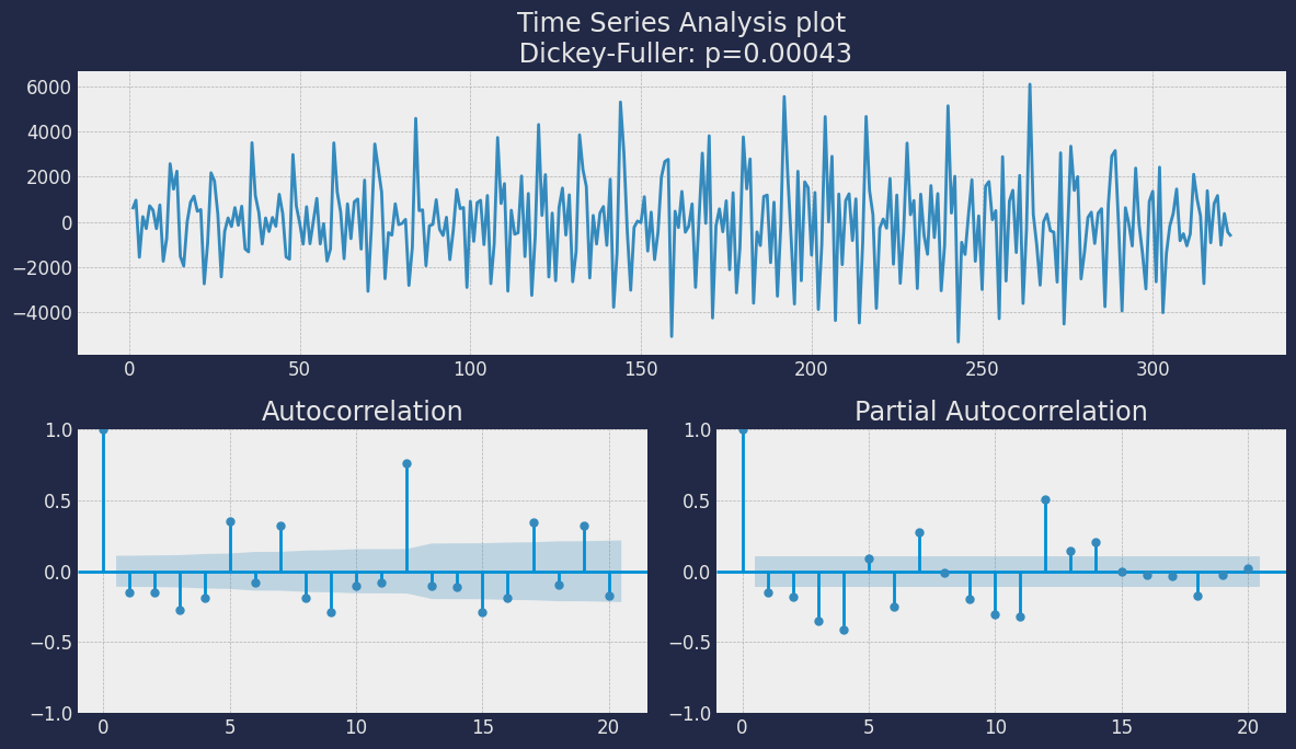 As you can see, based on the blue background shaded area of the graph,
the PACF shows the first, second, third, fourth, sixth, seventh, ninth,
and tenth etc. delay outside the shaded area. This means that it would
be interesting to also include these lags in the AR model.
### How many lags should we include?
Now, the **big question in time series analysis is always how many lags
to include**. This is called the order of the time series. The notation
is AR(1) for order 1 and AR(p) for order p.
The order is up to you. Theoretically speaking, you can base your order
on the PACF chart. Theory tells you to take the number of lags before
you get an autocorrelation of 0. All other lags should be 0.
In theory, you often see great charts where the first peak is very high
and the rest equal zero. In those cases, the choice is easy: you are
working with a very “pure” example of AR(1). Another common case is when
your autocorrelation starts high and slowly decreases to zero. In this
case, you should use all delays where the PACF is not yet zero.
However, in practice, it is not always that simple. Remember the famous
saying *“all models are wrong, but some are useful”*. It is very rare to
find cases that fit an AR model perfectly. In general, the
autoregression process can help explain part of the variation of a
variable, but not all.
In practice, you will try to select the number of lags that gives your
model the best predictive performance. The best predictive performance
is often not defined by looking at autocorrelation plots: those plots
give you a theoretical estimate. However, predictive performance is best
defined by model evaluation and benchmarking, using the techniques you
have seen in Module 2. Later in this module, we will see how to use
model evaluation to choose a performance order for the AR model. But
before we get into that, it’s time to dig into the exact definition of
the AR model.
## Split the data into training and testing
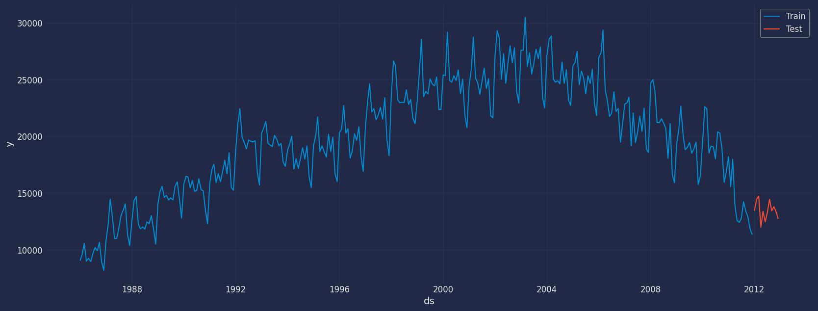
Let’s divide our data into sets 1. Data to train our `AutoRegressive`
model 2. Data to test our model
For the test data we will use the last 12 months to test and evaluate
the performance of our model.
```python theme={null}
train = df[df.ds<='2011-12-01']
test = df[df.ds>'2011-12-01']
```
```python theme={null}
train.shape, test.shape
```
```text theme={null}
((312, 3), (12, 3))
```
Now let’s plot the training data and the test data.
```python theme={null}
sns.lineplot(train,x="ds", y="y", label="Train")
sns.lineplot(test, x="ds", y="y", label="Test")
plt.show()
```
As you can see, based on the blue background shaded area of the graph,
the PACF shows the first, second, third, fourth, sixth, seventh, ninth,
and tenth etc. delay outside the shaded area. This means that it would
be interesting to also include these lags in the AR model.
### How many lags should we include?
Now, the **big question in time series analysis is always how many lags
to include**. This is called the order of the time series. The notation
is AR(1) for order 1 and AR(p) for order p.
The order is up to you. Theoretically speaking, you can base your order
on the PACF chart. Theory tells you to take the number of lags before
you get an autocorrelation of 0. All other lags should be 0.
In theory, you often see great charts where the first peak is very high
and the rest equal zero. In those cases, the choice is easy: you are
working with a very “pure” example of AR(1). Another common case is when
your autocorrelation starts high and slowly decreases to zero. In this
case, you should use all delays where the PACF is not yet zero.
However, in practice, it is not always that simple. Remember the famous
saying *“all models are wrong, but some are useful”*. It is very rare to
find cases that fit an AR model perfectly. In general, the
autoregression process can help explain part of the variation of a
variable, but not all.
In practice, you will try to select the number of lags that gives your
model the best predictive performance. The best predictive performance
is often not defined by looking at autocorrelation plots: those plots
give you a theoretical estimate. However, predictive performance is best
defined by model evaluation and benchmarking, using the techniques you
have seen in Module 2. Later in this module, we will see how to use
model evaluation to choose a performance order for the AR model. But
before we get into that, it’s time to dig into the exact definition of
the AR model.
## Split the data into training and testing
Let’s divide our data into sets 1. Data to train our `AutoRegressive`
model 2. Data to test our model
For the test data we will use the last 12 months to test and evaluate
the performance of our model.
```python theme={null}
train = df[df.ds<='2011-12-01']
test = df[df.ds>'2011-12-01']
```
```python theme={null}
train.shape, test.shape
```
```text theme={null}
((312, 3), (12, 3))
```
Now let’s plot the training data and the test data.
```python theme={null}
sns.lineplot(train,x="ds", y="y", label="Train")
sns.lineplot(test, x="ds", y="y", label="Test")
plt.show()
```
 # Implementation of AutoRegressive with StatsForecast
### Load libraries
```python theme={null}
from statsforecast import StatsForecast
from statsforecast.models import AutoRegressive
```
### Instantiating Model
Import and instantiate the models. Setting the argument is sometimes
tricky. This article on [Seasonal
periods](https://robjhyndman.com/hyndsight/seasonal-periods/) by the
master, Rob Hyndmann, can be useful.season\_length.
**Method 1:** We use the lags parameter in an integer format, that is,
we put the lags we want to evaluate in the model.
```python theme={null}
season_length = 12 # Monthly data
horizon = len(test) # number of predictions biasadj=True, include_drift=True,
models2 = [AutoRegressive(lags=[14], include_mean=True)]
```
**Method 2:** We use the lags parameter in a list format, that is, we
put the lags that we want to evaluate in the model in the form of a list
as shown below.
```python theme={null}
season_length = 12 # Monthly data
horizon = len(test) # number of predictions
models = [AutoRegressive(lags=[3,4,6,7,9,10,11,12,13,14], include_mean=True)]
```
We fit the models by instantiating a new StatsForecast object with the
following parameters:
models: a list of models. Select the models you want from models and
import them.
* `freq:` a string indicating the frequency of the data. (See
[pandas’s available
frequencies](https://pandas.pydata.org/pandas-docs/stable/user_guide/timeseries.html#offset-aliases).)
* `n_jobs:` n\_jobs: int, number of jobs used in the parallel
processing, use -1 for all cores.
* `fallback_model:` a model to be used if a model fails.
Any settings are passed into the constructor. Then you call its fit
method and pass in the historical data frame.
```python theme={null}
sf = StatsForecast(models=models, freq='MS')
```
### Fit Model
```python theme={null}
sf.fit(df=train)
```
```text theme={null}
StatsForecast(models=[AutoRegressive])
```
Let’s see the results of our Theta model. We can observe it with the
following instruction:
```python theme={null}
result=sf.fitted_[0,0].model_
print(result.keys())
```
```text theme={null}
dict_keys(['coef', 'sigma2', 'var_coef', 'mask', 'loglik', 'aic', 'arma', 'residuals', 'code', 'n_cond', 'nobs', 'model', 'aicc', 'bic', 'xreg', 'lambda', 'x'])
```
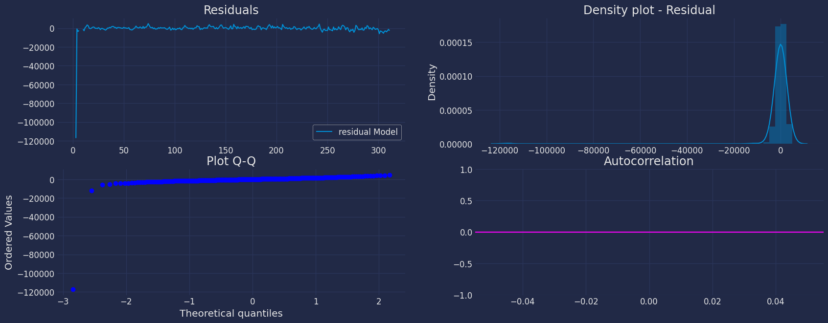
Let us now visualize the residuals of our models.
As we can see, the result obtained above has an output in a dictionary,
to extract each element from the dictionary we are going to use the
`.get()` function to extract the element and then we are going to save
it in a `pd.DataFrame()`.
```python theme={null}
residual=pd.DataFrame(result.get("residuals"), columns=["residual Model"])
residual
```
| | residual Model |
| --- | -------------- |
| 0 | -11998.537347 |
| 1 | NaN |
| 2 | NaN |
| ... | ... |
| 309 | -2718.312961 |
| 310 | -1306.795172 |
| 311 | -2713.284999 |
```python theme={null}
fig, axs = plt.subplots(nrows=2, ncols=2)
# plot[1,1]
residual.plot(ax=axs[0,0])
axs[0,0].set_title("Residuals");
# plot
sns.distplot(residual, ax=axs[0,1]);
axs[0,1].set_title("Density plot - Residual");
# plot
stats.probplot(residual["residual Model"], dist="norm", plot=axs[1,0])
axs[1,0].set_title('Plot Q-Q')
# plot
plot_acf(residual, lags=35, ax=axs[1,1],color="fuchsia")
axs[1,1].set_title("Autocorrelation");
plt.show();
```
# Implementation of AutoRegressive with StatsForecast
### Load libraries
```python theme={null}
from statsforecast import StatsForecast
from statsforecast.models import AutoRegressive
```
### Instantiating Model
Import and instantiate the models. Setting the argument is sometimes
tricky. This article on [Seasonal
periods](https://robjhyndman.com/hyndsight/seasonal-periods/) by the
master, Rob Hyndmann, can be useful.season\_length.
**Method 1:** We use the lags parameter in an integer format, that is,
we put the lags we want to evaluate in the model.
```python theme={null}
season_length = 12 # Monthly data
horizon = len(test) # number of predictions biasadj=True, include_drift=True,
models2 = [AutoRegressive(lags=[14], include_mean=True)]
```
**Method 2:** We use the lags parameter in a list format, that is, we
put the lags that we want to evaluate in the model in the form of a list
as shown below.
```python theme={null}
season_length = 12 # Monthly data
horizon = len(test) # number of predictions
models = [AutoRegressive(lags=[3,4,6,7,9,10,11,12,13,14], include_mean=True)]
```
We fit the models by instantiating a new StatsForecast object with the
following parameters:
models: a list of models. Select the models you want from models and
import them.
* `freq:` a string indicating the frequency of the data. (See
[pandas’s available
frequencies](https://pandas.pydata.org/pandas-docs/stable/user_guide/timeseries.html#offset-aliases).)
* `n_jobs:` n\_jobs: int, number of jobs used in the parallel
processing, use -1 for all cores.
* `fallback_model:` a model to be used if a model fails.
Any settings are passed into the constructor. Then you call its fit
method and pass in the historical data frame.
```python theme={null}
sf = StatsForecast(models=models, freq='MS')
```
### Fit Model
```python theme={null}
sf.fit(df=train)
```
```text theme={null}
StatsForecast(models=[AutoRegressive])
```
Let’s see the results of our Theta model. We can observe it with the
following instruction:
```python theme={null}
result=sf.fitted_[0,0].model_
print(result.keys())
```
```text theme={null}
dict_keys(['coef', 'sigma2', 'var_coef', 'mask', 'loglik', 'aic', 'arma', 'residuals', 'code', 'n_cond', 'nobs', 'model', 'aicc', 'bic', 'xreg', 'lambda', 'x'])
```
Let us now visualize the residuals of our models.
As we can see, the result obtained above has an output in a dictionary,
to extract each element from the dictionary we are going to use the
`.get()` function to extract the element and then we are going to save
it in a `pd.DataFrame()`.
```python theme={null}
residual=pd.DataFrame(result.get("residuals"), columns=["residual Model"])
residual
```
| | residual Model |
| --- | -------------- |
| 0 | -11998.537347 |
| 1 | NaN |
| 2 | NaN |
| ... | ... |
| 309 | -2718.312961 |
| 310 | -1306.795172 |
| 311 | -2713.284999 |
```python theme={null}
fig, axs = plt.subplots(nrows=2, ncols=2)
# plot[1,1]
residual.plot(ax=axs[0,0])
axs[0,0].set_title("Residuals");
# plot
sns.distplot(residual, ax=axs[0,1]);
axs[0,1].set_title("Density plot - Residual");
# plot
stats.probplot(residual["residual Model"], dist="norm", plot=axs[1,0])
axs[1,0].set_title('Plot Q-Q')
# plot
plot_acf(residual, lags=35, ax=axs[1,1],color="fuchsia")
axs[1,1].set_title("Autocorrelation");
plt.show();
```
 ### Forecast Method
If you want to gain speed in productive settings where you have multiple
series or models we recommend using the `StatsForecast.forecast` method
instead of `.fit` and `.predict`.
The main difference is that the `.forecast` doest not store the fitted
values and is highly scalable in distributed environments.
The forecast method takes two arguments: forecasts next `h` (horizon)
and `level`.
* `h (int):` represents the forecast h steps into the future. In this
case, 12 months ahead.
* `level (list of floats):` this optional parameter is used for
probabilistic forecasting. Set the level (or confidence percentile)
of your prediction interval. For example, `level=[90]` means that
the model expects the real value to be inside that interval 90% of
the times.
The forecast object here is a new data frame that includes a column with
the name of the model and the y hat values, as well as columns for the
uncertainty intervals. Depending on your computer, this step should take
around 1min. (If you want to speed things up to a couple of seconds,
remove the AutoModels like `ARIMA` and `Theta`)
```python theme={null}
# Prediction
Y_hat = sf.forecast(df=train, h=horizon, fitted=True)
Y_hat
```
| | unique\_id | ds | AutoRegressive |
| --- | ---------- | ---------- | -------------- |
| 0 | 1 | 2012-01-01 | 15905.582031 |
| 1 | 1 | 2012-02-01 | 13597.894531 |
| 2 | 1 | 2012-03-01 | 15488.883789 |
| ... | ... | ... | ... |
| 9 | 1 | 2012-10-01 | 14087.901367 |
| 10 | 1 | 2012-11-01 | 13274.105469 |
| 11 | 1 | 2012-12-01 | 12498.226562 |
```python theme={null}
values=sf.forecast_fitted_values()
values.head()
```
| | unique\_id | ds | y | AutoRegressive |
| - | ---------- | ---------- | ------- | -------------- |
| 0 | 1 | 1986-01-01 | 9034.0 | 21032.537109 |
| 1 | 1 | 1986-02-01 | 9596.0 | NaN |
| 2 | 1 | 1986-03-01 | 10558.0 | NaN |
| 3 | 1 | 1986-04-01 | 9002.0 | 126172.937500 |
| 4 | 1 | 1986-05-01 | 9239.0 | 10020.040039 |
Adding 95% confidence interval with the forecast method
```python theme={null}
sf.forecast(df=train, h=horizon, level=[95])
```
| | unique\_id | ds | AutoRegressive | AutoRegressive-lo-95 | AutoRegressive-hi-95 |
| --- | ---------- | ---------- | -------------- | -------------------- | -------------------- |
| 0 | 1 | 2012-01-01 | 15905.582031 | 2119.586426 | 29691.578125 |
| 1 | 1 | 2012-02-01 | 13597.894531 | -188.101135 | 27383.890625 |
| 2 | 1 | 2012-03-01 | 15488.883789 | 1702.888062 | 29274.878906 |
| ... | ... | ... | ... | ... | ... |
| 9 | 1 | 2012-10-01 | 14087.901367 | -1050.068359 | 29225.871094 |
| 10 | 1 | 2012-11-01 | 13274.105469 | -1886.973145 | 28435.183594 |
| 11 | 1 | 2012-12-01 | 12498.226562 | -2675.547607 | 27672.001953 |
```python theme={null}
# Merge the forecasts with the true values
Y_hat1 = test.merge(Y_hat, how='left', on=['unique_id', 'ds'])
Y_hat1
```
| | ds | y | unique\_id | AutoRegressive |
| --- | ---------- | ----- | ---------- | -------------- |
| 0 | 2012-01-01 | 13427 | 1 | 15905.582031 |
| 1 | 2012-02-01 | 14447 | 1 | 13597.894531 |
| 2 | 2012-03-01 | 14717 | 1 | 15488.883789 |
| ... | ... | ... | ... | ... |
| 9 | 2012-10-01 | 13795 | 1 | 14087.901367 |
| 10 | 2012-11-01 | 13352 | 1 | 13274.105469 |
| 11 | 2012-12-01 | 12716 | 1 | 12498.226562 |
```python theme={null}
sf.plot(train, Y_hat1)
```
### Forecast Method
If you want to gain speed in productive settings where you have multiple
series or models we recommend using the `StatsForecast.forecast` method
instead of `.fit` and `.predict`.
The main difference is that the `.forecast` doest not store the fitted
values and is highly scalable in distributed environments.
The forecast method takes two arguments: forecasts next `h` (horizon)
and `level`.
* `h (int):` represents the forecast h steps into the future. In this
case, 12 months ahead.
* `level (list of floats):` this optional parameter is used for
probabilistic forecasting. Set the level (or confidence percentile)
of your prediction interval. For example, `level=[90]` means that
the model expects the real value to be inside that interval 90% of
the times.
The forecast object here is a new data frame that includes a column with
the name of the model and the y hat values, as well as columns for the
uncertainty intervals. Depending on your computer, this step should take
around 1min. (If you want to speed things up to a couple of seconds,
remove the AutoModels like `ARIMA` and `Theta`)
```python theme={null}
# Prediction
Y_hat = sf.forecast(df=train, h=horizon, fitted=True)
Y_hat
```
| | unique\_id | ds | AutoRegressive |
| --- | ---------- | ---------- | -------------- |
| 0 | 1 | 2012-01-01 | 15905.582031 |
| 1 | 1 | 2012-02-01 | 13597.894531 |
| 2 | 1 | 2012-03-01 | 15488.883789 |
| ... | ... | ... | ... |
| 9 | 1 | 2012-10-01 | 14087.901367 |
| 10 | 1 | 2012-11-01 | 13274.105469 |
| 11 | 1 | 2012-12-01 | 12498.226562 |
```python theme={null}
values=sf.forecast_fitted_values()
values.head()
```
| | unique\_id | ds | y | AutoRegressive |
| - | ---------- | ---------- | ------- | -------------- |
| 0 | 1 | 1986-01-01 | 9034.0 | 21032.537109 |
| 1 | 1 | 1986-02-01 | 9596.0 | NaN |
| 2 | 1 | 1986-03-01 | 10558.0 | NaN |
| 3 | 1 | 1986-04-01 | 9002.0 | 126172.937500 |
| 4 | 1 | 1986-05-01 | 9239.0 | 10020.040039 |
Adding 95% confidence interval with the forecast method
```python theme={null}
sf.forecast(df=train, h=horizon, level=[95])
```
| | unique\_id | ds | AutoRegressive | AutoRegressive-lo-95 | AutoRegressive-hi-95 |
| --- | ---------- | ---------- | -------------- | -------------------- | -------------------- |
| 0 | 1 | 2012-01-01 | 15905.582031 | 2119.586426 | 29691.578125 |
| 1 | 1 | 2012-02-01 | 13597.894531 | -188.101135 | 27383.890625 |
| 2 | 1 | 2012-03-01 | 15488.883789 | 1702.888062 | 29274.878906 |
| ... | ... | ... | ... | ... | ... |
| 9 | 1 | 2012-10-01 | 14087.901367 | -1050.068359 | 29225.871094 |
| 10 | 1 | 2012-11-01 | 13274.105469 | -1886.973145 | 28435.183594 |
| 11 | 1 | 2012-12-01 | 12498.226562 | -2675.547607 | 27672.001953 |
```python theme={null}
# Merge the forecasts with the true values
Y_hat1 = test.merge(Y_hat, how='left', on=['unique_id', 'ds'])
Y_hat1
```
| | ds | y | unique\_id | AutoRegressive |
| --- | ---------- | ----- | ---------- | -------------- |
| 0 | 2012-01-01 | 13427 | 1 | 15905.582031 |
| 1 | 2012-02-01 | 14447 | 1 | 13597.894531 |
| 2 | 2012-03-01 | 14717 | 1 | 15488.883789 |
| ... | ... | ... | ... | ... |
| 9 | 2012-10-01 | 13795 | 1 | 14087.901367 |
| 10 | 2012-11-01 | 13352 | 1 | 13274.105469 |
| 11 | 2012-12-01 | 12716 | 1 | 12498.226562 |
```python theme={null}
sf.plot(train, Y_hat1)
```
 ### Predict method with confidence interval
To generate forecasts use the predict method.
The predict method takes two arguments: forecasts the next `h` (for
horizon) and `level`.
* `h (int):` represents the forecast h steps into the future. In this
case, 12 months ahead.
* `level (list of floats):` this optional parameter is used for
probabilistic forecasting. Set the level (or confidence percentile)
of your prediction interval. For example, `level=[95]` means that
the model expects the real value to be inside that interval 95% of
the times.
The forecast object here is a new data frame that includes a column with
the name of the model and the y hat values, as well as columns for the
uncertainty intervals.
This step should take less than 1 second.
```python theme={null}
sf.predict(h=horizon)
```
| | unique\_id | ds | AutoRegressive |
| --- | ---------- | ---------- | -------------- |
| 0 | 1 | 2012-01-01 | 15905.582031 |
| 1 | 1 | 2012-02-01 | 13597.894531 |
| 2 | 1 | 2012-03-01 | 15488.883789 |
| ... | ... | ... | ... |
| 9 | 1 | 2012-10-01 | 14087.901367 |
| 10 | 1 | 2012-11-01 | 13274.105469 |
| 11 | 1 | 2012-12-01 | 12498.226562 |
```python theme={null}
forecast_df = sf.predict(h=horizon, level=[95])
forecast_df
```
| | unique\_id | ds | AutoRegressive | AutoRegressive-lo-95 | AutoRegressive-hi-95 |
| --- | ---------- | ---------- | -------------- | -------------------- | -------------------- |
| 0 | 1 | 2012-01-01 | 15905.582031 | 2119.586426 | 29691.578125 |
| 1 | 1 | 2012-02-01 | 13597.894531 | -188.101135 | 27383.890625 |
| 2 | 1 | 2012-03-01 | 15488.883789 | 1702.888062 | 29274.878906 |
| ... | ... | ... | ... | ... | ... |
| 9 | 1 | 2012-10-01 | 14087.901367 | -1050.068359 | 29225.871094 |
| 10 | 1 | 2012-11-01 | 13274.105469 | -1886.973145 | 28435.183594 |
| 11 | 1 | 2012-12-01 | 12498.226562 | -2675.547607 | 27672.001953 |
```python theme={null}
sf.plot(train, test.merge(forecast_df), level=[95])
```
### Predict method with confidence interval
To generate forecasts use the predict method.
The predict method takes two arguments: forecasts the next `h` (for
horizon) and `level`.
* `h (int):` represents the forecast h steps into the future. In this
case, 12 months ahead.
* `level (list of floats):` this optional parameter is used for
probabilistic forecasting. Set the level (or confidence percentile)
of your prediction interval. For example, `level=[95]` means that
the model expects the real value to be inside that interval 95% of
the times.
The forecast object here is a new data frame that includes a column with
the name of the model and the y hat values, as well as columns for the
uncertainty intervals.
This step should take less than 1 second.
```python theme={null}
sf.predict(h=horizon)
```
| | unique\_id | ds | AutoRegressive |
| --- | ---------- | ---------- | -------------- |
| 0 | 1 | 2012-01-01 | 15905.582031 |
| 1 | 1 | 2012-02-01 | 13597.894531 |
| 2 | 1 | 2012-03-01 | 15488.883789 |
| ... | ... | ... | ... |
| 9 | 1 | 2012-10-01 | 14087.901367 |
| 10 | 1 | 2012-11-01 | 13274.105469 |
| 11 | 1 | 2012-12-01 | 12498.226562 |
```python theme={null}
forecast_df = sf.predict(h=horizon, level=[95])
forecast_df
```
| | unique\_id | ds | AutoRegressive | AutoRegressive-lo-95 | AutoRegressive-hi-95 |
| --- | ---------- | ---------- | -------------- | -------------------- | -------------------- |
| 0 | 1 | 2012-01-01 | 15905.582031 | 2119.586426 | 29691.578125 |
| 1 | 1 | 2012-02-01 | 13597.894531 | -188.101135 | 27383.890625 |
| 2 | 1 | 2012-03-01 | 15488.883789 | 1702.888062 | 29274.878906 |
| ... | ... | ... | ... | ... | ... |
| 9 | 1 | 2012-10-01 | 14087.901367 | -1050.068359 | 29225.871094 |
| 10 | 1 | 2012-11-01 | 13274.105469 | -1886.973145 | 28435.183594 |
| 11 | 1 | 2012-12-01 | 12498.226562 | -2675.547607 | 27672.001953 |
```python theme={null}
sf.plot(train, test.merge(forecast_df), level=[95])
```
 ## Cross-validation
In previous steps, we’ve taken our historical data to predict the
future. However, to asses its accuracy we would also like to know how
the model would have performed in the past. To assess the accuracy and
robustness of your models on your data perform Cross-Validation.
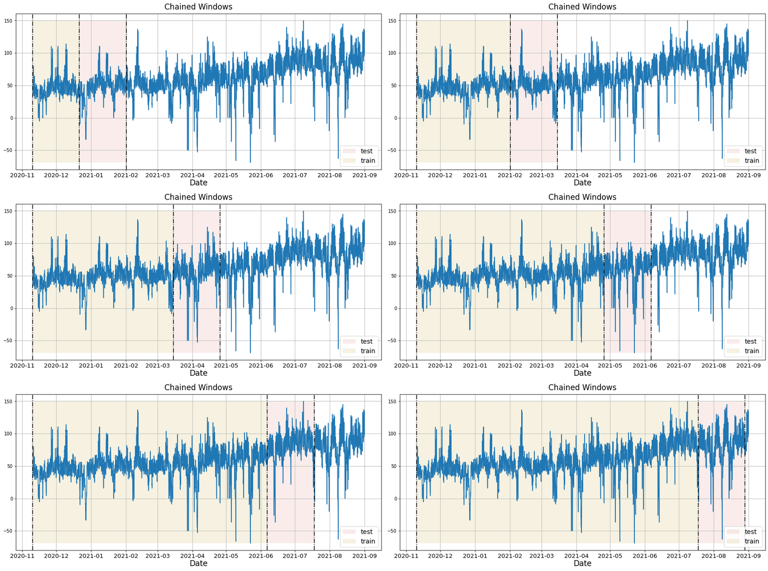
With time series data, Cross Validation is done by defining a sliding
window across the historical data and predicting the period following
it. This form of cross-validation allows us to arrive at a better
estimation of our model’s predictive abilities across a wider range of
temporal instances while also keeping the data in the training set
contiguous as is required by our models.
The following graph depicts such a Cross Validation Strategy:
### Perform time series cross-validation
Cross-validation of time series models is considered a best practice but
most implementations are very slow. The statsforecast library implements
cross-validation as a distributed operation, making the process less
time-consuming to perform. If you have big datasets you can also perform
Cross Validation in a distributed cluster using Ray, Dask or Spark.
In this case, we want to evaluate the performance of each model for the
last 5 months `(n_windows=5)`, forecasting every second months
`(step_size=12)`. Depending on your computer, this step should take
around 1 min.
The cross\_validation method from the StatsForecast class takes the
following arguments.
* `df:` training data frame
* `h (int):` represents h steps into the future that are being
forecasted. In this case, 12 months ahead.
* `step_size (int):` step size between each window. In other words:
how often do you want to run the forecasting processes.
* `n_windows(int):` number of windows used for cross validation. In
other words: what number of forecasting processes in the past do you
want to evaluate.
```python theme={null}
crossvalidation_df = sf.cross_validation(df=train,
h=horizon,
step_size=6,
n_windows=5)
```
The crossvaldation\_df object is a new data frame that includes the
following columns:
* `unique_id:` series identifier
* `ds:` datestamp or temporal index
* `cutoff:` the last datestamp or temporal index for the n\_windows.
* `y:` true value
* `"model":` columns with the model’s name and fitted value.
```python theme={null}
crossvalidation_df
```
| | unique\_id | ds | cutoff | y | AutoRegressive |
| --- | ---------- | ---------- | ---------- | ------- | -------------- |
| 0 | 1 | 2009-01-01 | 2008-12-01 | 19262.0 | 24295.837891 |
| 1 | 1 | 2009-02-01 | 2008-12-01 | 20658.0 | 23993.947266 |
| 2 | 1 | 2009-03-01 | 2008-12-01 | 22660.0 | 21201.121094 |
| ... | ... | ... | ... | ... | ... |
| 57 | 1 | 2011-10-01 | 2010-12-01 | 12893.0 | 19349.708984 |
| 58 | 1 | 2011-11-01 | 2010-12-01 | 11843.0 | 16899.849609 |
| 59 | 1 | 2011-12-01 | 2010-12-01 | 11321.0 | 18159.574219 |
We’ll now plot the forecast for each cutoff period. To make the plots
clearer, we’ll rename the actual values in each period.
```python theme={null}
from IPython.display import display
```
```python theme={null}
crossvalidation_df.rename(columns = {'y' : 'actual'}, inplace = True) # rename actual values
cutoff = crossvalidation_df['cutoff'].unique()
for k in range(len(cutoff)):
cv = crossvalidation_df[crossvalidation_df['cutoff'] == cutoff[k]]
display(StatsForecast.plot(df, cv.loc[:, cv.columns != 'cutoff']))
```
## Cross-validation
In previous steps, we’ve taken our historical data to predict the
future. However, to asses its accuracy we would also like to know how
the model would have performed in the past. To assess the accuracy and
robustness of your models on your data perform Cross-Validation.
With time series data, Cross Validation is done by defining a sliding
window across the historical data and predicting the period following
it. This form of cross-validation allows us to arrive at a better
estimation of our model’s predictive abilities across a wider range of
temporal instances while also keeping the data in the training set
contiguous as is required by our models.
The following graph depicts such a Cross Validation Strategy:

### Perform time series cross-validation
Cross-validation of time series models is considered a best practice but
most implementations are very slow. The statsforecast library implements
cross-validation as a distributed operation, making the process less
time-consuming to perform. If you have big datasets you can also perform
Cross Validation in a distributed cluster using Ray, Dask or Spark.
In this case, we want to evaluate the performance of each model for the
last 5 months `(n_windows=5)`, forecasting every second months
`(step_size=12)`. Depending on your computer, this step should take
around 1 min.
The cross\_validation method from the StatsForecast class takes the
following arguments.
* `df:` training data frame
* `h (int):` represents h steps into the future that are being
forecasted. In this case, 12 months ahead.
* `step_size (int):` step size between each window. In other words:
how often do you want to run the forecasting processes.
* `n_windows(int):` number of windows used for cross validation. In
other words: what number of forecasting processes in the past do you
want to evaluate.
```python theme={null}
crossvalidation_df = sf.cross_validation(df=train,
h=horizon,
step_size=6,
n_windows=5)
```
The crossvaldation\_df object is a new data frame that includes the
following columns:
* `unique_id:` series identifier
* `ds:` datestamp or temporal index
* `cutoff:` the last datestamp or temporal index for the n\_windows.
* `y:` true value
* `"model":` columns with the model’s name and fitted value.
```python theme={null}
crossvalidation_df
```
| | unique\_id | ds | cutoff | y | AutoRegressive |
| --- | ---------- | ---------- | ---------- | ------- | -------------- |
| 0 | 1 | 2009-01-01 | 2008-12-01 | 19262.0 | 24295.837891 |
| 1 | 1 | 2009-02-01 | 2008-12-01 | 20658.0 | 23993.947266 |
| 2 | 1 | 2009-03-01 | 2008-12-01 | 22660.0 | 21201.121094 |
| ... | ... | ... | ... | ... | ... |
| 57 | 1 | 2011-10-01 | 2010-12-01 | 12893.0 | 19349.708984 |
| 58 | 1 | 2011-11-01 | 2010-12-01 | 11843.0 | 16899.849609 |
| 59 | 1 | 2011-12-01 | 2010-12-01 | 11321.0 | 18159.574219 |
We’ll now plot the forecast for each cutoff period. To make the plots
clearer, we’ll rename the actual values in each period.
```python theme={null}
from IPython.display import display
```
```python theme={null}
crossvalidation_df.rename(columns = {'y' : 'actual'}, inplace = True) # rename actual values
cutoff = crossvalidation_df['cutoff'].unique()
for k in range(len(cutoff)):
cv = crossvalidation_df[crossvalidation_df['cutoff'] == cutoff[k]]
display(StatsForecast.plot(df, cv.loc[:, cv.columns != 'cutoff']))
```




 ## Model Evaluation
Now we are going to evaluate our model with the results of the
predictions, we will use different types of metrics MAE, MAPE, MASE,
RMSE, SMAPE to evaluate the accuracy.
```python theme={null}
from functools import partial
import utilsforecast.losses as ufl
from utilsforecast.evaluation import evaluate
```
```python theme={null}
evaluate(
test.merge(Y_hat),
metrics=[ufl.mae, ufl.mape, partial(ufl.mase, seasonality=season_length), ufl.rmse, ufl.smape],
train_df=train,
agg_fn='mean',
)
```
| | metric | AutoRegressive |
| - | ------ | -------------- |
| 0 | mae | 962.023763 |
| 1 | mape | 0.072733 |
| 2 | mase | 0.601808 |
| 3 | rmse | 1195.013050 |
| 4 | smape | 0.034858 |
## References
1. [Changquan Huang • Alla Petukhina. Springer series (2022). Applied
Time Series Analysis and Forecasting with
Python.](https://link.springer.com/book/10.1007/978-3-031-13584-2)
2. [Jose A. Fiorucci, Tiago R. Pellegrini, Francisco Louzada, Fotios
Petropoulos, Anne B. Koehler (2016). “Models for optimising the
theta method and their relationship to state space models”.
International Journal of
Forecasting](https://www.sciencedirect.com/science/article/pii/S0169207016300243).
3. [Nixtla AutoRegressive
API](../../src/core/models.html#autoregressive)
4. [Pandas available
frequencies](https://pandas.pydata.org/pandas-docs/stable/user_guide/timeseries.html#offset-aliases).
5. [Rob J. Hyndman and George Athanasopoulos (2018). “Forecasting
Principles and Practice (3rd
ed)”](https://otexts.com/fpp3/tscv.html)
6. [Seasonal periods- Rob J
Hyndman](https://robjhyndman.com/hyndsight/seasonal-periods/).
## Model Evaluation
Now we are going to evaluate our model with the results of the
predictions, we will use different types of metrics MAE, MAPE, MASE,
RMSE, SMAPE to evaluate the accuracy.
```python theme={null}
from functools import partial
import utilsforecast.losses as ufl
from utilsforecast.evaluation import evaluate
```
```python theme={null}
evaluate(
test.merge(Y_hat),
metrics=[ufl.mae, ufl.mape, partial(ufl.mase, seasonality=season_length), ufl.rmse, ufl.smape],
train_df=train,
agg_fn='mean',
)
```
| | metric | AutoRegressive |
| - | ------ | -------------- |
| 0 | mae | 962.023763 |
| 1 | mape | 0.072733 |
| 2 | mase | 0.601808 |
| 3 | rmse | 1195.013050 |
| 4 | smape | 0.034858 |
## References
1. [Changquan Huang • Alla Petukhina. Springer series (2022). Applied
Time Series Analysis and Forecasting with
Python.](https://link.springer.com/book/10.1007/978-3-031-13584-2)
2. [Jose A. Fiorucci, Tiago R. Pellegrini, Francisco Louzada, Fotios
Petropoulos, Anne B. Koehler (2016). “Models for optimising the
theta method and their relationship to state space models”.
International Journal of
Forecasting](https://www.sciencedirect.com/science/article/pii/S0169207016300243).
3. [Nixtla AutoRegressive
API](../../src/core/models.html#autoregressive)
4. [Pandas available
frequencies](https://pandas.pydata.org/pandas-docs/stable/user_guide/timeseries.html#offset-aliases).
5. [Rob J. Hyndman and George Athanasopoulos (2018). “Forecasting
Principles and Practice (3rd
ed)”](https://otexts.com/fpp3/tscv.html)
6. [Seasonal periods- Rob J
Hyndman](https://robjhyndman.com/hyndsight/seasonal-periods/).