> ## Documentation Index
> Fetch the complete documentation index at: https://nixtlaverse.nixtla.io/llms.txt
> Use this file to discover all available pages before exploring further.
# AutoETS Model
> Step-by-step guide on using the `AutoETS Model` with `Statsforecast`.
During this walkthrough, we will become familiar with the main
`StatsForecast` class and some relevant methods such as
`StatsForecast.plot`, `StatsForecast.forecast` and
`StatsForecast.cross_validation` in other.
The text in this article is largely taken from [Rob J. Hyndman and
George Athanasopoulos (2018). “Forecasting Principles and Practice (3rd
ed)”](https://otexts.com/fpp3/tscv.html).
## Table of Contents
* [Introduction](#introduction)
* [ETS Models](#model)
* [ETS Estimation](#estimation)
* [Model Selection](#selection)
* [Loading libraries and data](#loading)
* [Explore data with the plot method](#plotting)
* [Split the data into training and testing](#splitting)
* [Implementation of AutoETS with StatsForecast](#implementation)
* [Cross-validation](#cross_validate)
* [Model evaluation](#evaluate)
* [References](#references)
## Introduction
Automatic forecasts of large numbers of univariate time series are often
needed in business. It is common to have over one thousand product lines
that need forecasting at least monthly. Even when a smaller number of
forecasts are required, there may be nobody suitably trained in the use
of time series models to produce them. In these circumstances, an
automatic forecasting algorithm is an essential tool. Automatic
forecasting algorithms must determine an appropriate time series model,
estimate the parameters and compute the forecasts. They must be robust
to unusual time series patterns, and applicable to large numbers of
series without user intervention. The most popular automatic forecasting
algorithms are based on either exponential smoothing or ARIMA models.
# Exponential smoothing
Although exponential smoothing methods have been around since the 1950s,
a modelling framework incorporating procedures for model selection was
not developed until relatively recently. `Ord, Koehler`, and
`Snyder (1997), Hyndman, Koehler, Snyder, and Grose (2002)` and
`Hyndman, Koehler, Ord`, and `Snyder (2005b)` have shown that all
exponential smoothing methods (including non-linear methods) are optimal
forecasts from innovations state space models.
Exponential smoothing methods were originally classified by
`Pegels’ (1969) taxonomy`. This was later extended by
`Gardner (1985), modified by Hyndman et al. (2002)`, and extended again
by `Taylor (2003)`, giving a total of fifteen methods seen in the
following table.
| Trend Component | Seasonal Component |
| --------------- | ------------------ |
| Component | N(None)) | A (Additive) | M (Multiplicative) |
| -------------------------- | -------- | ------------ | ------------------ |
| N (None) | (N,N) | (N,A) | (N,M) |
| A (Additive) | (A,N) | (A,A) | (A,M) |
| Ad (Additive damped) | (Ad,N) | (Ad,A) | (Ad,M) |
| M (Multiplicative) | (M,N ) | (M,A ) | (M,M) |
| Md (Multiplicative damped) | (Md,N ) | ( Md,A) | (Md,M) |
Some of these methods are better known under other names. For example,
cell `(N,N)` describes the **simple exponential smoothing (or SES)
method**, cell `(A,N)` describes **Holt’s linear method**, and cell
`(Ad,N)` describes **the damped trend method**. The **additive
Holt-Winters’ method** is given by cell `(A,A)` and the **multiplicative
Holt-Winters’ method** is given by cell `(A,M)`. The other cells
correspond to less commonly used but analogous methods.
### Point forecasts for all methods
We denote the observed time series by $y_1,y_2,...,y_n$. A forecast of
$y_{t+h}$ based on all of the data up to time $t$ is denoted by
$\hat y_{t+h|t}$. To illustrate the method, we give the point forecasts
and updating equation for method `(A,A)`, the he Holt-Winters’ additive
method:
where $m$ is the length of seasonality (e.g., the number of months or
quarters in a year), $\ell_{t}$ represents the level of the series,
$b_t$ denotes the growth, $s_t$ is the seasonal component,
$\hat y_{t+h|t}$ is the forecast for $h$ periods ahead, and
$h_{m}^{+} = [(h − 1) mod \ m] + 1$. To use method (1), we need values
for the initial states $\ell_{0}$, $b_0$ and $s_{1−m}, . . . , s_0$, and
for the smoothing parameters $\alpha, \beta^{*}$ and $\gamma$. All of
these will be estimated from the observed data.
Equation (1c) is slightly different from the usual Holt-Winters
equations such as those in Makridakis et al. (1998) or Bowerman,
O’Connell, and Koehler (2005). These authors replace (1c) with
$s_{t} = \gamma^* (y_{t}-\ell_{t})+ (1-\gamma^*)s_{t-m}.$
If $\ell_{t}$ is substituted using (1a), we obtain
$s_{t} = \gamma^*(1-\alpha) (y_{t}-\ell_{t-1}-b_{t-1})+ [1-\gamma^*(1-\alpha)]s_{t-m},$
Thus, we obtain identical forecasts using this approach by replacing
$\gamma$ in (1c) with $\gamma^{*} (1-\alpha)$. The modification given in
(1c) was proposed by Ord et al. (1997) to make the state space
formulation simpler. It is equivalent to Archibald’s (1990) variation of
the Holt-Winters’ method.
### Innovations state space models
For each exponential smoothing method in [Other ETS
models](https://otexts.com/fpp3/ets.html) , Hyndman et al. (2008b)
describe two possible innovations state space models, one corresponding
to a model with additive errors and the other to a model with
multiplicative errors. If the same parameter values are used, these two
models give equivalent point forecasts, although different prediction
intervals. Thus there are 30 potential models described in this
classification.
Historically, the nature of the error component has often been ignored,
because the distinction between additive and multiplicative errors makes
no difference to point forecasts.
We are careful to distinguish exponential smoothing methods from the
underlying state space models. An exponential smoothing method is an
algorithm for producing point forecasts only. The underlying stochastic
state space model gives the same point forecasts, but also provides a
framework for computing prediction intervals and other properties.
To distinguish the models with additive and multiplicative errors, we
add an extra letter to the front of the method notation. The triplet
`(E,T,S)` refers to the three components: error, trend and seasonality.
So the model `ETS(A,A,N)` has additive errors, additive trend and no
seasonality—in other words, this is Holt’s linear method with additive
errors. Similarly, `ETS(M,Md,M)` refers to a model with multiplicative
errors, a damped multiplicative trend and multiplicative seasonality.
The notation `ETS(·,·,·)` helps in remembering the order in which the
components are specified.
Once a model is specified, we can study the probability distribution of
future values of the series and find, for example, the conditional mean
of a future observation given knowledge of the past. We denote this as
$\mu_{t+h|t} = E(y_{t+h | xt})$, where xt contains the unobserved
components such as $\ell_t$, $b_t$ and $s_t$. For $h = 1$ we use
$\mu_t ≡ \mu_{t+1|t}$ as a shorthand notation. For many models, these
conditional means will be identical to the point forecasts given in
Table [Other ETS models](https://otexts.com/fpp3/ets.html), so that
$\mu_{t+h|t} = \hat y_{t+h|t}$. However, for other models (those with
multiplicative trend or multiplicative seasonality), the conditional
mean and the point forecast will differ slightly for $h ≥ 2$.
We illustrate these ideas using the damped trend method of Gardner and
McKenzie (1985).
Each model consists of a measurement equation that describes the
observed data, and some state equations that describe how the unobserved
components or states (level, trend, seasonal) change over time. Hence,
these are referred to as state space models.
For each method there exist two models: one with additive errors and one
with multiplicative errors. The point forecasts produced by the models
are identical if they use the same smoothing parameter values. They
will, however, generate different prediction intervals.
To distinguish between a model with additive errors and one with
multiplicative errors (and also to distinguish the models from the
methods), we add a third letter to the classification of in the above
Table. We label each state space model as `ETS(⋅,.,.)` for (Error,
Trend, Seasonal). This label can also be thought of as ExponenTial
Smoothing. Using the same notation as in the above Table, the
possibilities for each component (or state) are: `Error ={ A,M }`,
`Trend ={N,A,Ad}` and `Seasonal ={ N,A,M }`.
### **ETS(A,N,N): simple exponential smoothing with additive errors**
Recall the component form of simple exponential smoothing:
If we re-arrange the smoothing equation for the level, we get the “error
correction” form,
where $e_{t}=y_{t}-\ell_{t-1}=y_{t}-\hat{y}_{t|t-1}$ s the residual at
time $t$.
The training data errors lead to the adjustment of the estimated level
throughout the smoothing process for $t=1,\dots,T$. For example, if the
error at time $t$ is negative, then $y_t < \hat{y}_{t|t-1}$ and so the
level at time $t-1$ has been over-estimated. The new level $\ell_{t}$ is
then the previous level $\ell_{t-1}$ adjusted downwards. The closer
$\alpha$ is to one, the “rougher” the estimate of the level (large
adjustments take place). The smaller the $\alpha$, the “smoother” the
level (small adjustments take place).
We can also write $y_t = \ell_{t-1} + e_t$, so that each observation can
be represented by the previous level plus an error. To make this into an
innovations state space model, all we need to do is specify the
probability distribution for $e_t$. For a model with additive errors, we
assume that residuals (the one-step training errors) $e_t$ are normally
distributed white noise with mean 0 and variance $\sigma^2$. A
short-hand notation for this is
$e_t = \varepsilon_t\sim\text{NID}(0,\sigma^2)$; NID stands for
“normally and independently distributed”.
Then the equations of the model can be written as
We refer to (2) as the measurement (or observation) equation and (3) as
the state (or transition) equation. These two equations, together with
the statistical distribution of the errors, form a fully specified
statistical model. Specifically, these constitute an innovations state
space model underlying simple exponential smoothing.
The term “innovations” comes from the fact that all equations use the
same random error process, $\varepsilon_t$. For the same reason, this
formulation is also referred to as a “single source of error” model.
There are alternative multiple source of error formulations which we do
not present here.
The measurement equation shows the relationship between the observations
and the unobserved states. In this case, observation $y_t$ is a linear
function of the level $\ell_{t-1}$, the predictable part of $y_t$, and
the error $\varepsilon_t$, the unpredictable part of $y_t$. For other
innovations state space models, this relationship may be nonlinear.
The state equation shows the evolution of the state through time. The
influence of the smoothing parameter $\alpha$ is the same as for the
methods discussed earlier. For example, $\alpha$ governs the amount of
change in successive levels: high values of $\alpha$ allow rapid changes
in the level; low values of $\alpha$ lead to smooth changes. If
$\alpha=0$, the level of the series does not change over time; if
$\alpha=1$, the model reduces to a random walk model,
$y_t=y_{t-1}+\varepsilon_t$.
### **ETS(M,N,N): simple exponential smoothing with multiplicative errors**
In a similar fashion, we can specify models with multiplicative errors
by writing the one-step-ahead training errors as relative errors
$\varepsilon_t = \frac{y_t-\hat{y}_{t|t-1}}{\hat{y}_{t|t-1}}$
where $\varepsilon_t \sim \text{NID}(0,\sigma^2)$. Substituting
$\hat{y}_{t|t-1}=\ell_{t-1}$ gives
$y_t = \ell_{t-1}+\ell_{t-1}\varepsilon_t$ and
$e_t = y_t - \hat{y}_{t|t-1} = \ell_{t-1}\varepsilon_t$.
Then we can write the multiplicative form of the state space model as
### **ETS(A,A,N): Holt’s linear method with additive errors**
For this model, we assume that the one-step-ahead training errors are
given by
$\varepsilon_t=y_t-\ell_{t-1}-b_{t-1} \sim \text{NID}(0,\sigma^2)$
Substituting this into the error correction equations for Holt’s linear
method we obtain
where for simplicity we have set $\beta=\alpha \beta^*$.
### **ETS(M,A,N): Holt’s linear method with multiplicative errors**
Specifying one-step-ahead training errors as relative errors such that
$\varepsilon_t=\frac{y_t-(\ell_{t-1}+b_{t-1})}{(\ell_{t-1}+b_{t-1})}$
and following an approach similar to that used above, the innovations
state space model underlying Holt’s linear method with multiplicative
errors is specified as
where again $\beta=\alpha \beta^*$ and
$\varepsilon_t \sim \text{NID}(0,\sigma^2)$.
## Estimating ETS models
An alternative to estimating the parameters by minimising the sum of
squared errors is to maximise the “likelihood”. The likelihood is the
probability of the data arising from the specified model. Thus, a large
likelihood is associated with a good model. For an additive error model,
maximising the likelihood (assuming normally distributed errors) gives
the same results as minimising the sum of squared errors. However,
different results will be obtained for multiplicative error models. In
this section, we will estimate the smoothing parameters
$\alpha, \beta, \gamma$ and $\phi$ and the initial states
$\ell_0, b_0, s_0,s_{-1},\dots,s_{-m+1}$, by maximising the likelihood.
The possible values that the smoothing parameters can take are
restricted. Traditionally, the parameters have been constrained to lie
between 0 and 1 so that the equations can be interpreted as weighted
averages. That is, $0< \alpha,\beta^*,\gamma^*,\phi<1$. For the state
space models, we have set $\beta=\alpha\beta^*$ and
$\gamma=(1-\alpha)\gamma^*$. Therefore, the traditional restrictions
translate to $0< \alpha <1, 0 < \beta < \alpha$ and
$0< \gamma < 1-\alpha$. In practice, the damping parameter $\phi$ is
usually constrained further to prevent numerical difficulties in
estimating the model.
Another way to view the parameters is through a consideration of the
mathematical properties of the state space models. The parameters are
constrained in order to prevent observations in the distant past having
a continuing effect on current forecasts. This leads to some
admissibility constraints on the parameters, which are usually (but not
always) less restrictive than the traditional constraints region
`(Hyndman et al., 2008, pp. 149-161)`. For example, for the `ETS(A,N,N)`
model, the traditional parameter region is $0< \alpha <1$ but the
admissible region is $0< \alpha <2$. For the `ETS(A,A,N)` model, the
traditional parameter region is $0<\alpha<1$ and $0<\beta<\alpha$ but
the admissible region is $0<\alpha<2$ and $0<\beta<4-2\alpha$.
## Model selection
A great advantage of the `ETS` statistical framework is that information
criteria can be used for model selection. The `AIC, AIC_c` and `BIC`,
can be used here to determine which of the `ETS` models is most
appropriate for a given time series.
For `ETS` models, Akaike’s Information Criterion (`AIC)` is defined as
$\text{AIC} = -2\log(L) + 2k,$
where $L$ is the likelihood of the model and $k$ is the total number of
parameters and initial states that have been estimated (including the
residual variance).
The `AIC` corrected for small sample bias `(AIC_c)` is defined as
$AIC_c = AIC + \frac{2k(k+1)}{T-k-1}$
and the Bayesian Information Criterion `(BIC)` is
$\text{BIC} = \text{AIC} + k[\log(T)-2]$
Three of the combinations of (Error, Trend, Seasonal) can lead to
numerical difficulties. Specifically, the models that can cause such
instabilities are `ETS(A,N,M), ETS(A,A,M)`, and `ETS(A,Ad,M)`, due to
division by values potentially close to zero in the state equations. We
normally do not consider these particular combinations when selecting a
model.
Models with multiplicative errors are useful when the data are strictly
positive, but are not numerically stable when the data contain zeros or
negative values. Therefore, multiplicative error models will not be
considered if the time series is not strictly positive. In that case,
only the six fully additive models will be applied.
## Loading libraries and data
> **Tip**
>
> Statsforecast will be needed. To install, see
> [instructions](../getting-started/installation.html).
Next, we import plotting libraries and configure the plotting style.
```python theme={null}
import numpy as np
import pandas as pd
```
```python theme={null}
import matplotlib.pyplot as plt
import seaborn as sns
from statsmodels.graphics.tsaplots import plot_acf
from statsmodels.graphics.tsaplots import plot_pacf
plt.style.use('fivethirtyeight')
plt.rcParams['lines.linewidth'] = 1.5
dark_style = {
'figure.facecolor': '#212946',
'axes.facecolor': '#212946',
'savefig.facecolor':'#212946',
'axes.grid': True,
'axes.grid.which': 'both',
'axes.spines.left': False,
'axes.spines.right': False,
'axes.spines.top': False,
'axes.spines.bottom': False,
'grid.color': '#2A3459',
'grid.linewidth': '1',
'text.color': '0.9',
'axes.labelcolor': '0.9',
'xtick.color': '0.9',
'ytick.color': '0.9',
'font.size': 12 }
plt.rcParams.update(dark_style)
from pylab import rcParams
rcParams['figure.figsize'] = (18,7)
```
### Read Data
```python theme={null}
df = pd.read_csv("https://raw.githubusercontent.com/Naren8520/Serie-de-tiempo-con-Machine-Learning/main/Data/Esperanza_vida.csv", usecols=[1,2])
df.head()
```
| | year | value |
| - | ---------- | --------- |
| 0 | 1960-01-01 | 69.123902 |
| 1 | 1961-01-01 | 69.760244 |
| 2 | 1962-01-01 | 69.149756 |
| 3 | 1963-01-01 | 69.248049 |
| 4 | 1964-01-01 | 70.311707 |
The input to StatsForecast is always a data frame in long format with
three columns: unique\_id, ds and y:
* The `unique_id` (string, int or category) represents an identifier
for the series.
* The `ds` (datestamp) column should be of a format expected by
Pandas, ideally YYYY-MM-DD for a date or YYYY-MM-DD HH:MM:SS for a
timestamp.
* The `y` (numeric) represents the measurement we wish to forecast.
```python theme={null}
df["unique_id"]="1"
df.columns=["ds", "y", "unique_id"]
df.head()
```
| | ds | y | unique\_id |
| - | ---------- | --------- | ---------- |
| 0 | 1960-01-01 | 69.123902 | 1 |
| 1 | 1961-01-01 | 69.760244 | 1 |
| 2 | 1962-01-01 | 69.149756 | 1 |
| 3 | 1963-01-01 | 69.248049 | 1 |
| 4 | 1964-01-01 | 70.311707 | 1 |
```python theme={null}
print(df.dtypes)
```
```text theme={null}
ds object
y float64
unique_id object
dtype: object
```
We need to convert the `ds` from `object` type to datetime.
```python theme={null}
df["ds"] = pd.to_datetime(df["ds"])
```
## Explore data with the plot method
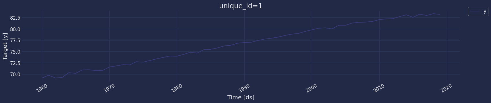
Plot some series using the plot method from the StatsForecast class.
This method prints a random series from the dataset and is useful for
basic EDA.
```python theme={null}
from statsforecast import StatsForecast
StatsForecast.plot(df)
```
 ## Autocorrelation plots
```python theme={null}
fig, axs = plt.subplots(nrows=1, ncols=2)
plot_acf(df["y"], lags=20, ax=axs[0],color="fuchsia")
axs[0].set_title("Autocorrelation");
# Plot
plot_pacf(df["y"], lags=20, ax=axs[1],color="lime")
axs[1].set_title('Partial Autocorrelation')
plt.show();
```
## Autocorrelation plots
```python theme={null}
fig, axs = plt.subplots(nrows=1, ncols=2)
plot_acf(df["y"], lags=20, ax=axs[0],color="fuchsia")
axs[0].set_title("Autocorrelation");
# Plot
plot_pacf(df["y"], lags=20, ax=axs[1],color="lime")
axs[1].set_title('Partial Autocorrelation')
plt.show();
```
 ### Decomposition of the time series
How to decompose a time series and why?
In time series analysis to forecast new values, it is very important to
know past data. More formally, we can say that it is very important to
know the patterns that values follow over time. There can be many
reasons that cause our forecast values to fall in the wrong direction.
Basically, a time series consists of four components. The variation of
those components causes the change in the pattern of the time series.
These components are:
* **Level:** This is the primary value that averages over time.
* **Trend:** The trend is the value that causes increasing or
decreasing patterns in a time series.
* **Seasonality:** This is a cyclical event that occurs in a time
series for a short time and causes short-term increasing or
decreasing patterns in a time series.
* **Residual/Noise:** These are the random variations in the time
series.
Combining these components over time leads to the formation of a time
series. Most time series consist of level and noise/residual and trend
or seasonality are optional values.
If seasonality and trend are part of the time series, then there will be
effects on the forecast value. As the pattern of the forecasted time
series may be different from the previous time series.
The combination of the components in time series can be of two types: \*
Additive \* Multiplicative
### Additive time series
If the components of the time series are added to make the time series.
Then the time series is called the additive time series. By
visualization, we can say that the time series is additive if the
increasing or decreasing pattern of the time series is similar
throughout the series. The mathematical function of any additive time
series can be represented by:
$y(t) = level + Trend + seasonality + noise$
### Multiplicative time series
If the components of the time series are multiplicative together, then
the time series is called a multiplicative time series. For
visualization, if the time series is having exponential growth or
decline with time, then the time series can be considered as the
multiplicative time series. The mathematical function of the
multiplicative time series can be represented as.
$y(t) = Level * Trend * seasonality * Noise$
```python theme={null}
from statsmodels.tsa.seasonal import seasonal_decompose
a = seasonal_decompose(df["y"], model = "add", period=1)
a.plot();
```
### Decomposition of the time series
How to decompose a time series and why?
In time series analysis to forecast new values, it is very important to
know past data. More formally, we can say that it is very important to
know the patterns that values follow over time. There can be many
reasons that cause our forecast values to fall in the wrong direction.
Basically, a time series consists of four components. The variation of
those components causes the change in the pattern of the time series.
These components are:
* **Level:** This is the primary value that averages over time.
* **Trend:** The trend is the value that causes increasing or
decreasing patterns in a time series.
* **Seasonality:** This is a cyclical event that occurs in a time
series for a short time and causes short-term increasing or
decreasing patterns in a time series.
* **Residual/Noise:** These are the random variations in the time
series.
Combining these components over time leads to the formation of a time
series. Most time series consist of level and noise/residual and trend
or seasonality are optional values.
If seasonality and trend are part of the time series, then there will be
effects on the forecast value. As the pattern of the forecasted time
series may be different from the previous time series.
The combination of the components in time series can be of two types: \*
Additive \* Multiplicative
### Additive time series
If the components of the time series are added to make the time series.
Then the time series is called the additive time series. By
visualization, we can say that the time series is additive if the
increasing or decreasing pattern of the time series is similar
throughout the series. The mathematical function of any additive time
series can be represented by:
$y(t) = level + Trend + seasonality + noise$
### Multiplicative time series
If the components of the time series are multiplicative together, then
the time series is called a multiplicative time series. For
visualization, if the time series is having exponential growth or
decline with time, then the time series can be considered as the
multiplicative time series. The mathematical function of the
multiplicative time series can be represented as.
$y(t) = Level * Trend * seasonality * Noise$
```python theme={null}
from statsmodels.tsa.seasonal import seasonal_decompose
a = seasonal_decompose(df["y"], model = "add", period=1)
a.plot();
```
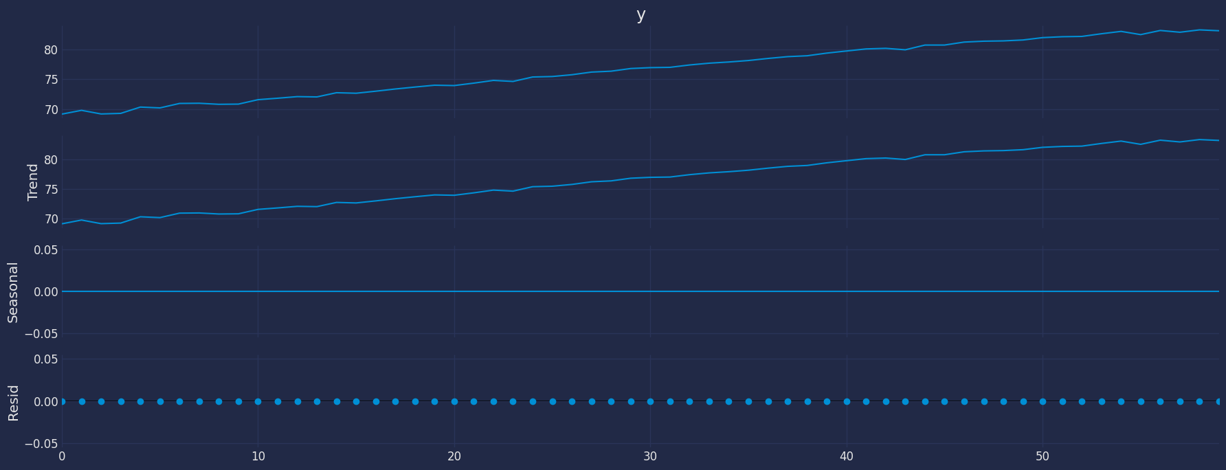 Breaking down a time series into its components helps us to identify the
behavior of the time series we are analyzing. In addition, it helps us
to know what type of models we can apply, for our example of the Life
expectancy data set, we can observe that our time series shows an
increasing trend throughout the year, on the other hand, it can be
observed also that the time series has no seasonality.
By looking at the previous graph and knowing each of the components, we
can get an idea of which model we can apply: \* We have trend \* There
is no seasonality
## Split the data into training and testing
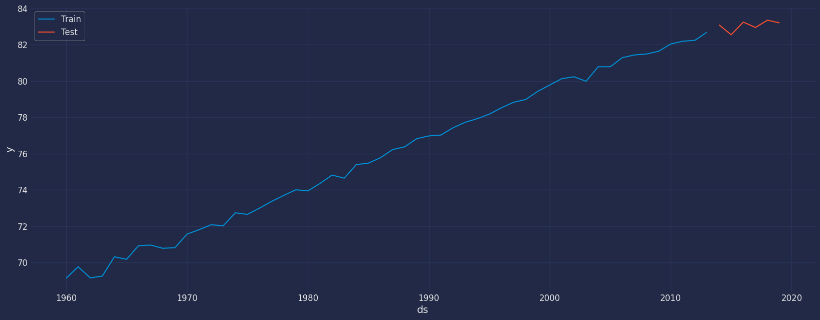
Let’s divide our data into sets
1. Data to train our model.
2. Data to test our model.
For the test data we will use the last 6 years to test and evaluate the
performance of our model.
```python theme={null}
train = df[df.ds<='2013-01-01']
test = df[df.ds>'2013-01-01']
```
```python theme={null}
train.shape, test.shape
```
```text theme={null}
((54, 3), (6, 3))
```
```python theme={null}
sns.lineplot(train,x="ds", y="y", label="Train")
sns.lineplot(test, x="ds", y="y", label="Test")
plt.show()
```
Breaking down a time series into its components helps us to identify the
behavior of the time series we are analyzing. In addition, it helps us
to know what type of models we can apply, for our example of the Life
expectancy data set, we can observe that our time series shows an
increasing trend throughout the year, on the other hand, it can be
observed also that the time series has no seasonality.
By looking at the previous graph and knowing each of the components, we
can get an idea of which model we can apply: \* We have trend \* There
is no seasonality
## Split the data into training and testing
Let’s divide our data into sets
1. Data to train our model.
2. Data to test our model.
For the test data we will use the last 6 years to test and evaluate the
performance of our model.
```python theme={null}
train = df[df.ds<='2013-01-01']
test = df[df.ds>'2013-01-01']
```
```python theme={null}
train.shape, test.shape
```
```text theme={null}
((54, 3), (6, 3))
```
```python theme={null}
sns.lineplot(train,x="ds", y="y", label="Train")
sns.lineplot(test, x="ds", y="y", label="Test")
plt.show()
```
 ## Implementation of AutoETS with StatsForecast
```python theme={null}
from statsforecast import StatsForecast
from statsforecast.models import AutoETS
```
### Instantiate Model
```python theme={null}
sf = StatsForecast(models=[AutoETS(model="AZN")], freq='YS')
```
### Fit the Model
```python theme={null}
sf.fit(df=train)
```
```text theme={null}
StatsForecast(models=[AutoETS])
```
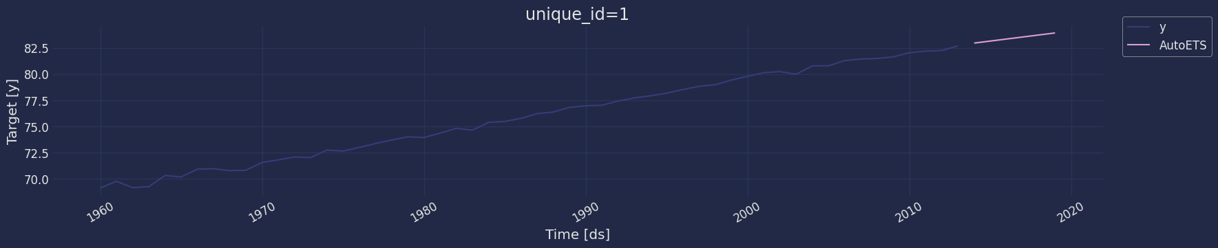
### Model Prediction
```python theme={null}
y_hat = sf.predict(h=6)
y_hat
```
| | unique\_id | ds | AutoETS |
| - | ---------- | ---------- | --------- |
| 0 | 1 | 2014-01-01 | 82.952553 |
| 1 | 1 | 2015-01-01 | 83.146150 |
| 2 | 1 | 2016-01-01 | 83.339747 |
| 3 | 1 | 2017-01-01 | 83.533344 |
| 4 | 1 | 2018-01-01 | 83.726940 |
| 5 | 1 | 2019-01-01 | 83.920537 |
```python theme={null}
sf.plot(train, y_hat)
```
## Implementation of AutoETS with StatsForecast
```python theme={null}
from statsforecast import StatsForecast
from statsforecast.models import AutoETS
```
### Instantiate Model
```python theme={null}
sf = StatsForecast(models=[AutoETS(model="AZN")], freq='YS')
```
### Fit the Model
```python theme={null}
sf.fit(df=train)
```
```text theme={null}
StatsForecast(models=[AutoETS])
```
### Model Prediction
```python theme={null}
y_hat = sf.predict(h=6)
y_hat
```
| | unique\_id | ds | AutoETS |
| - | ---------- | ---------- | --------- |
| 0 | 1 | 2014-01-01 | 82.952553 |
| 1 | 1 | 2015-01-01 | 83.146150 |
| 2 | 1 | 2016-01-01 | 83.339747 |
| 3 | 1 | 2017-01-01 | 83.533344 |
| 4 | 1 | 2018-01-01 | 83.726940 |
| 5 | 1 | 2019-01-01 | 83.920537 |
```python theme={null}
sf.plot(train, y_hat)
```
 Let’s add a confidence interval to our forecast.
```python theme={null}
y_hat = sf.predict(h=6, level=[80,90,95])
y_hat
```
| | unique\_id | ds | AutoETS | AutoETS-lo-95 | AutoETS-lo-90 | AutoETS-lo-80 | AutoETS-hi-80 | AutoETS-hi-90 | AutoETS-hi-95 |
| - | ---------- | ---------- | --------- | ------------- | ------------- | ------------- | ------------- | ------------- | ------------- |
| 0 | 1 | 2014-01-01 | 82.952553 | 82.500416 | 82.573107 | 82.656916 | 83.248190 | 83.331999 | 83.404691 |
| 1 | 1 | 2015-01-01 | 83.146150 | 82.693437 | 82.766221 | 82.850137 | 83.442163 | 83.526078 | 83.598863 |
| 2 | 1 | 2016-01-01 | 83.339747 | 82.884744 | 82.957897 | 83.042237 | 83.637257 | 83.721597 | 83.794749 |
| 3 | 1 | 2017-01-01 | 83.533344 | 83.073235 | 83.147208 | 83.232495 | 83.834192 | 83.919479 | 83.993452 |
| 4 | 1 | 2018-01-01 | 83.726940 | 83.257894 | 83.333304 | 83.420247 | 84.033634 | 84.120577 | 84.195987 |
| 5 | 1 | 2019-01-01 | 83.920537 | 83.437859 | 83.515461 | 83.604931 | 84.236144 | 84.325614 | 84.403216 |
```python theme={null}
sf.plot(train, y_hat, level=[95])
```
Let’s add a confidence interval to our forecast.
```python theme={null}
y_hat = sf.predict(h=6, level=[80,90,95])
y_hat
```
| | unique\_id | ds | AutoETS | AutoETS-lo-95 | AutoETS-lo-90 | AutoETS-lo-80 | AutoETS-hi-80 | AutoETS-hi-90 | AutoETS-hi-95 |
| - | ---------- | ---------- | --------- | ------------- | ------------- | ------------- | ------------- | ------------- | ------------- |
| 0 | 1 | 2014-01-01 | 82.952553 | 82.500416 | 82.573107 | 82.656916 | 83.248190 | 83.331999 | 83.404691 |
| 1 | 1 | 2015-01-01 | 83.146150 | 82.693437 | 82.766221 | 82.850137 | 83.442163 | 83.526078 | 83.598863 |
| 2 | 1 | 2016-01-01 | 83.339747 | 82.884744 | 82.957897 | 83.042237 | 83.637257 | 83.721597 | 83.794749 |
| 3 | 1 | 2017-01-01 | 83.533344 | 83.073235 | 83.147208 | 83.232495 | 83.834192 | 83.919479 | 83.993452 |
| 4 | 1 | 2018-01-01 | 83.726940 | 83.257894 | 83.333304 | 83.420247 | 84.033634 | 84.120577 | 84.195987 |
| 5 | 1 | 2019-01-01 | 83.920537 | 83.437859 | 83.515461 | 83.604931 | 84.236144 | 84.325614 | 84.403216 |
```python theme={null}
sf.plot(train, y_hat, level=[95])
```
 ### Forecast method
Memory Efficient Exponential Smoothing predictions.
This method avoids memory burden due from object storage. It is
analogous to fit\_predict without storing information. It assumes you
know the forecast horizon in advance.
```python theme={null}
y_hat = sf.forecast(df=train, h=6, fitted=True)
y_hat
```
| | unique\_id | ds | AutoETS |
| - | ---------- | ---------- | --------- |
| 0 | 1 | 2014-01-01 | 82.952553 |
| 1 | 1 | 2015-01-01 | 83.146150 |
| 2 | 1 | 2016-01-01 | 83.339747 |
| 3 | 1 | 2017-01-01 | 83.533344 |
| 4 | 1 | 2018-01-01 | 83.726940 |
| 5 | 1 | 2019-01-01 | 83.920537 |
### In sample predictions
Access fitted Exponential Smoothing insample predictions.
```python theme={null}
sf.forecast_fitted_values()
```
| | unique\_id | ds | y | AutoETS |
| --- | ---------- | ---------- | --------- | --------- |
| 0 | 1 | 1960-01-01 | 69.123902 | 69.005305 |
| 1 | 1 | 1961-01-01 | 69.760244 | 69.237346 |
| 2 | 1 | 1962-01-01 | 69.149756 | 69.495763 |
| ... | ... | ... | ... | ... |
| 51 | 1 | 2011-01-01 | 82.187805 | 82.348633 |
| 52 | 1 | 2012-01-01 | 82.239024 | 82.561938 |
| 53 | 1 | 2013-01-01 | 82.690244 | 82.758963 |
## Model Evaluation
Now we are going to evaluate our model with the results of the
predictions, we will use different types of metrics MAE, MAPE, MASE,
RMSE, SMAPE to evaluate the accuracy.
```python theme={null}
from functools import partial
import utilsforecast.losses as ufl
from utilsforecast.evaluation import evaluate
```
```python theme={null}
evaluate(
y_hat.merge(test),
metrics=[ufl.mae, ufl.mape, partial(ufl.mase, seasonality=1), ufl.rmse, ufl.smape],
train_df=train,
)
```
| | unique\_id | metric | AutoETS |
| - | ---------- | ------ | -------- |
| 0 | 1 | mae | 0.421060 |
| 1 | 1 | mape | 0.005073 |
| 2 | 1 | mase | 1.340056 |
| 3 | 1 | rmse | 0.483558 |
| 4 | 1 | smape | 0.002528 |
## References
1. [Nixtla AutoETS API](../../src/core/models.html#autoets)
2. [Rob J. Hyndman and George Athanasopoulos (2018). “Forecasting
Principles and Practice (3rd
ed)”](https://otexts.com/fpp3/tscv.html).
### Forecast method
Memory Efficient Exponential Smoothing predictions.
This method avoids memory burden due from object storage. It is
analogous to fit\_predict without storing information. It assumes you
know the forecast horizon in advance.
```python theme={null}
y_hat = sf.forecast(df=train, h=6, fitted=True)
y_hat
```
| | unique\_id | ds | AutoETS |
| - | ---------- | ---------- | --------- |
| 0 | 1 | 2014-01-01 | 82.952553 |
| 1 | 1 | 2015-01-01 | 83.146150 |
| 2 | 1 | 2016-01-01 | 83.339747 |
| 3 | 1 | 2017-01-01 | 83.533344 |
| 4 | 1 | 2018-01-01 | 83.726940 |
| 5 | 1 | 2019-01-01 | 83.920537 |
### In sample predictions
Access fitted Exponential Smoothing insample predictions.
```python theme={null}
sf.forecast_fitted_values()
```
| | unique\_id | ds | y | AutoETS |
| --- | ---------- | ---------- | --------- | --------- |
| 0 | 1 | 1960-01-01 | 69.123902 | 69.005305 |
| 1 | 1 | 1961-01-01 | 69.760244 | 69.237346 |
| 2 | 1 | 1962-01-01 | 69.149756 | 69.495763 |
| ... | ... | ... | ... | ... |
| 51 | 1 | 2011-01-01 | 82.187805 | 82.348633 |
| 52 | 1 | 2012-01-01 | 82.239024 | 82.561938 |
| 53 | 1 | 2013-01-01 | 82.690244 | 82.758963 |
## Model Evaluation
Now we are going to evaluate our model with the results of the
predictions, we will use different types of metrics MAE, MAPE, MASE,
RMSE, SMAPE to evaluate the accuracy.
```python theme={null}
from functools import partial
import utilsforecast.losses as ufl
from utilsforecast.evaluation import evaluate
```
```python theme={null}
evaluate(
y_hat.merge(test),
metrics=[ufl.mae, ufl.mape, partial(ufl.mase, seasonality=1), ufl.rmse, ufl.smape],
train_df=train,
)
```
| | unique\_id | metric | AutoETS |
| - | ---------- | ------ | -------- |
| 0 | 1 | mae | 0.421060 |
| 1 | 1 | mape | 0.005073 |
| 2 | 1 | mase | 1.340056 |
| 3 | 1 | rmse | 0.483558 |
| 4 | 1 | smape | 0.002528 |
## References
1. [Nixtla AutoETS API](../../src/core/models.html#autoets)
2. [Rob J. Hyndman and George Athanasopoulos (2018). “Forecasting
Principles and Practice (3rd
ed)”](https://otexts.com/fpp3/tscv.html).