> ## Documentation Index
> Fetch the complete documentation index at: https://nixtlaverse.nixtla.io/llms.txt
> Use this file to discover all available pages before exploring further.
# ARIMA Model
> Step-by-step guide on using the `ARIMA Model` with `Statsforecast`.
In this walkthrough, we will become familiar with the main
`StatsForecast` class and some relevant methods such as
`StatsForecast.plot`, `StatsForecast.forecast` and
`StatsForecast.cross_validation`.
The text in this article is largely taken from [Rob J. Hyndman and
George Athanasopoulos (2018). “Forecasting Principles and Practice (3rd
ed)”.](https://otexts.com/fpp3/tscv.html)
## Table of Contents
* [Introduction](#introduction)
* [ARIMA Models](#model)
* [The meaning of p, d and q in ARIMA model](#concepts)
* [AR and MA models](#ar_ma)
* [ARIMA model](#arima)
* [How to find the order of differencing (d) in ARIMA model](#order_d)
* [Loading libraries and data](#loading)
* [Explore data with the plot method](#plotting)
* [How to find the order of the AR term (p)](#order_p)
* [How to find the order of the MA term (q)](#order_q)
* [How to handle if a time series is slightly under or over
differenced](#differencing)
* [Implementation of ARIMA with StatsForecast](#implementation)
* [Cross-validation](#cross_validate)
* [Model evaluation](#evaluate)
* [References](#references)
## Introduction
* A **Time Series** is defined as a series of data points recorded at
different time intervals. The time order can be daily, monthly, or
even yearly.
* Time Series forecasting is the process of using a statistical model
to predict future values of a time series based on past results.
* We have discussed various aspects of **Time Series Forecasting** in
the previous notebook.
* Forecasting is the step where we want to predict the future values
the series is going to take. Forecasting a time series is often of
tremendous commercial value.
**Forecasting a time series can be broadly divided into two types.**
* If we use only the previous values of the time series to predict its
future values, it is called **Univariate Time Series Forecasting.**
* If we use predictors other than the series (like exogenous
variables) to forecast it is called **Multi Variate Time Series
Forecasting.**
* This notebook focuses on a particular type of forecasting method
called **ARIMA modeling.**
## Introduction to ARIMA Models
* **ARIMA** stands for **Autoregressive Integrated Moving Average
Model**. It belongs to a class of models that explains a given time
series based on its own past values -i.e.- its own lags and the
lagged forecast errors. The equation can be used to forecast future
values. Any ‘non-seasonal’ time series that exhibits patterns and is
not a random white noise can be modeled with ARIMA models.
* So, **ARIMA**, short for **AutoRegressive Integrated Moving
Average**, is a forecasting algorithm based on the idea that the
information in the past values of the time series can alone be used
to predict the future values.
* **ARIMA Models** are specified by three order parameters: (p, d, q),
where,
* p is the order of the AR term
* q is the order of the MA term
* d is the number of differencing required to make the time series
stationary
* **AR(p) Autoregression** - a regression model that utilizes the
dependent relationship between a current observation and
observations over a previous period. An auto regressive (AR(p))
component refers to the use of past values in the regression
equation for the time series.
* **I(d) Integration** - uses differencing of observations
(subtracting an observation from observation at the previous time
step) in order to make the time series stationary. Differencing
involves the subtraction of the current values of a series with its
previous values d number of times.
* **MA(q) Moving Average** - a model that uses the dependency between
an observation and a residual error from a moving average model
applied to lagged observations. A moving average component depicts
the error of the model as a combination of previous error terms. The
order q represents the number of terms to be included in the model.
### Types of ARIMA Model
* **ARIMA** : Non-seasonal Autoregressive Integrated Moving Averages
* **SARIMA** : Seasonal ARIMA
* **SARIMAX** : Seasonal ARIMA with exogenous variables
If a time series, has seasonal patterns, then we need to add seasonal
terms and it becomes SARIMA, short for **Seasonal ARIMA**.
## The meaning of p, d and q in ARIMA model
### The meaning of p
* `p` is the order of the **Auto Regressive (AR)** term. It refers to
the number of lags of Y to be used as predictors.
### The meaning of d
* The term **Auto Regressive**’ in ARIMA means it is a linear
regression model that uses its own lags as predictors. Linear
regression models, as we know, work best when the predictors are not
correlated and are independent of each other. So we need to make the
time series stationary.
* The most common approach to make the series stationary is to
difference it. That is, subtract the previous value from the current
value. Sometimes, depending on the complexity of the series, more
than one differencing may be needed.
* The value of d, therefore, is the minimum number of differencing
needed to make the series stationary. If the time series is already
stationary, then d = 0.
### The meaning of q
* **q** is the order of the **Moving Average (MA)** term. It refers to
the number of lagged forecast errors that should go into the ARIMA
Model.
## AR and MA models
### AR model
In an autoregression model, we forecast the variable of interest using a
linear combination of past values of the variable. The term
autoregression indicates that it is a regression of the variable against
itself.
Thus, an autoregressive model of order p can be written as
$$
\begin{equation}
y_{t} = c + \phi_{1}y_{t-1} + \phi_{2}y_{t-2} + \dots + \phi_{p}y_{t-p} + \varepsilon_{t} \tag{1}
\end{equation}
$$
where $\epsilon_t$ is white noise. This is like a multiple regression
but with lagged values of $y_t$ as predictors. We refer to this as an
AR( p) model, an autoregressive model of order p.
### MA model
Rather than using past values of the forecast variable in a regression,
a moving average model uses past forecast errors in a regression-like
model,
$$
\begin{equation}
y_{t} = c + \varepsilon_t + \theta_{1}\varepsilon_{t-1} + \theta_{2}\varepsilon_{t-2} + \dots + \theta_{q}\varepsilon_{t-q} \tag{2}
\end{equation}
$$
where $\epsilon_t$ is white noise. We refer to this as an MA(q) model, a
moving average model of order q. Of course, we do not observe the values
of\
$\epsilon_t$ , so it is not really a regression in the usual sense.
Notice that each value of yt can be thought of as a weighted moving
average of the past few forecast errors (although the coefficients will
not normally sum to one). However, moving average models should not be
confused with the moving average smoothing . A moving average model is
used for forecasting future values, while moving average smoothing is
used for estimating the trend-cycle of past values.
Thus, we have discussed AR and MA Models respectively.
## ARIMA model
If we combine differencing with autoregression and a moving average
model, we obtain a non-seasonal ARIMA model. ARIMA is an acronym for
AutoRegressive Integrated Moving Average (in this context, “integration”
is the reverse of differencing). The full model can be written as
where $y'_{t}$ is the differenced series (it may have been differenced
more than once). The “predictors” on the right hand side include both
lagged values of $y_t$ and lagged errors. We call this an ARIMA(p,d,q)
model, where
| | |
| - | ------------------------------------- |
| p | order of the autoregressive part |
| d | degree of first differencing involved |
| q | order of the moving average part |
The same stationarity and invertibility conditions that are used for
autoregressive and moving average models also apply to an ARIMA model.
Many of the models we have already discussed are special cases of the
ARIMA model, as shown in Table
| Model | p d q | Differenced | Method |
| -------------------------- | ----- | --------------------------------------------------------------------------------------------------------------------------------- | ------------------------------------------ |
| Arima(0,0,0) | 0 0 0 | $y_t=Y_t$ | White noise |
| ARIMA (0,1,0) | 0 1 0 | $y_t = Y_t - Y_{t-1}$ | Random walk |
| ARIMA (0,2,0) | 0 2 0 | $y_t = Y_t - 2Y_{t-1} + Y_{t-2}$ | Constant |
| ARIMA (1,0,0) | 1 0 0 | $\hat Y_t = \mu + \Phi_1 Y_{t-1} + \epsilon$ | AR(1): AR(1): First-order regression model |
| ARIMA (2, 0, 0) | 2 0 0 | $\hat Y_t = \Phi_0 + \Phi_1 Y_{t-1} + \Phi_2 Y_{t-2} + \epsilon$ | AR(2): Second-order regression model |
| ARIMA (1, 1, 0) | 1 1 0 | $\hat Y_t = \mu + Y_{t-1} + \Phi_1 (Y_{t-1}- Y_{t-2})$ | Differenced first-order |
| autoregressive model | | | |
| ARIMA (0, 1, 1) | 0 1 1 | $\hat Y_t = Y_{t-1} - \Phi_1 e^{t-1}$ | Simple exponential |
| smoothing | | | |
| ARIMA (0, 0, 1) | 0 0 1 | $\hat Y_t = \mu_0+ \epsilon_t - \omega_1 \epsilon_{t-1}$ | MA(1): First-order |
| regression model | | | |
| ARIMA (0, 0, 2) | 0 0 2 | $\hat Y_t = \mu_0+ \epsilon_t - \omega_1 \epsilon_{t-1} - \omega_2 \epsilon_{t-2}$ | MA(2): Second-order |
| regression model | | | |
| ARIMA (1, 0, 1) | 1 0 1 | $\hat Y_t = \Phi_0 + \Phi_1 Y_{t-1}+ \epsilon_t - \omega_1 \epsilon_{t-1}$ | ARMA model |
| ARIMA (1, 1, 1) | 1 1 1 | $\Delta Y_t = \Phi_1 Y_{t-1} + \epsilon_t - \omega_1 \epsilon_{t-1}$ | ARIMA model |
| ARIMA (1, 1, 2) | 1 1 2 | $\hat Y_t = Y_{t-1} + \Phi_1 (Y_{t-1} - Y_{t-2} )- \Theta_1 e_{t-1} - \Theta_1 e_{t-1}$ Damped-trend linear Exponential smoothing | |
| ARIMA (0, 2, 1) OR (0,2,2) | 0 2 1 | $\hat Y_t = 2 Y_{t-1} - Y_{t-2} - \Theta_1 e_{t-1} - \Theta_2 e_{t-2}$ | Linear exponential smoothing |
Once we start combining components in this way to form more complicated
models, it is much easier to work with the backshift notation. For
example, the above equation can be written in backshift notation as
### ARIMA model in words
Predicted Yt = Constant + Linear combination Lags of Y (upto p lags) +
Linear Combination of Lagged forecast errors (upto q lags)
## How to find the order of differencing (d) in ARIMA model
* As stated earlier, the purpose of differencing is to make the time
series stationary. But we should be careful to not over-difference
the series. An over differenced series may still be stationary,
which in turn will affect the model parameters.
* So we should determine the right order of differencing. The right
order of differencing is the minimum differencing required to get a
near-stationary series which roams around a defined mean and the ACF
plot reaches to zero fairly quick.
* If the autocorrelations are positive for many number of lags (10 or
more), then the series needs further differencing. On the other
hand, if the lag 1 autocorrelation itself is too negative, then the
series is probably over-differenced.
* If we can’t really decide between two orders of differencing, then
we go with the order that gives the least standard deviation in the
differenced series.
* Now, we will explain these concepts with the help of an example as
follows:
* First, I will check if the series is stationary using the
**Augmented Dickey Fuller test (ADF Test)**, from the
statsmodels package. The reason being is that we need
differencing only if the series is non-stationary. Else, no
differencing is needed, that is, d=0.
* The null hypothesis (Ho) of the ADF test is that the time series
is non-stationary. So, if the p-value of the test is less than
the significance level (0.05) then we reject the null hypothesis
and infer that the time series is indeed stationary.
* So, in our case, if P Value > 0.05 we go ahead with finding the
order of differencing.
## Loading libraries and data
> **Tip**
>
> Statsforecast will be needed. To install, see
> [instructions](../getting-started/installation.html).
Next, we import plotting libraries and configure the plotting style.
```python theme={null}
import matplotlib.pyplot as plt
plt.style.use('fivethirtyeight')
plt.rcParams['lines.linewidth'] = 1.5
dark_style = {
'figure.facecolor': '#212946',
'axes.facecolor': '#212946',
'savefig.facecolor':'#212946',
'axes.grid': True,
'axes.grid.which': 'both',
'axes.spines.left': False,
'axes.spines.right': False,
'axes.spines.top': False,
'axes.spines.bottom': False,
'grid.color': '#2A3459',
'grid.linewidth': '1',
'text.color': '0.9',
'axes.labelcolor': '0.9',
'xtick.color': '0.9',
'ytick.color': '0.9',
'font.size': 12 }
plt.rcParams.update(dark_style)
from pylab import rcParams
rcParams['figure.figsize'] = (18,7)
```
### Read data
```python theme={null}
import pandas as pd
import numpy as np
df = pd.read_csv("https://raw.githubusercontent.com/Naren8520/Serie-de-tiempo-con-Machine-Learning/main/Data/Esperanza_vida.csv", usecols=[1,2])
df.head()
```
| | year | value |
| - | ---------- | --------- |
| 0 | 1960-01-01 | 69.123902 |
| 1 | 1961-01-01 | 69.760244 |
| 2 | 1962-01-01 | 69.149756 |
| 3 | 1963-01-01 | 69.248049 |
| 4 | 1964-01-01 | 70.311707 |
The input to StatsForecast is always a data frame in long format with
three columns: unique\_id, ds and y:
* The `unique_id` (string, int or category) represents an identifier
for the series.
* The `ds` (datestamp) column should be of a format expected by
Pandas, ideally YYYY-MM-DD for a date or YYYY-MM-DD HH:MM:SS for a
timestamp.
* The `y` (numeric) represents the measurement we wish to forecast.
```python theme={null}
df["unique_id"]="1"
df.columns=["ds", "y", "unique_id"]
df.head()
```
| | ds | y | unique\_id |
| - | ---------- | --------- | ---------- |
| 0 | 1960-01-01 | 69.123902 | 1 |
| 1 | 1961-01-01 | 69.760244 | 1 |
| 2 | 1962-01-01 | 69.149756 | 1 |
| 3 | 1963-01-01 | 69.248049 | 1 |
| 4 | 1964-01-01 | 70.311707 | 1 |
```python theme={null}
print(df.dtypes)
```
```text theme={null}
ds object
y float64
unique_id object
dtype: object
```
We need to convert `ds` from the `object` type to datetime.
```python theme={null}
df["ds"] = pd.to_datetime(df["ds"])
```
## Explore data with the plot method
Plot a series using the plot method from the StatsForecast class. This
method prints a random series from the dataset and is useful for basic
EDA.
```python theme={null}
from statsforecast import StatsForecast
StatsForecast.plot(df)
```
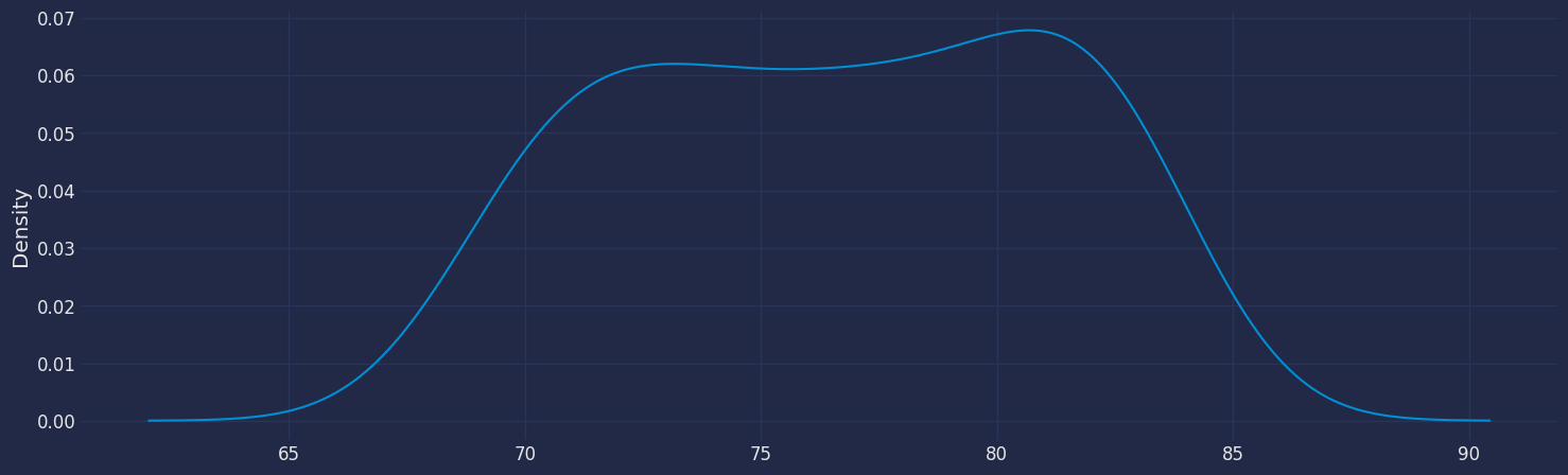
 Looking at the plot we can observe there is an upward trend over the
period of time.
```python theme={null}
df["y"].plot(kind='kde',figsize = (16,5))
df["y"].describe()
```
```text theme={null}
count 60.000000
mean 76.632439
std 4.495279
...
50% 76.895122
75% 80.781098
max 83.346341
Name: y, Length: 8, dtype: float64
```
Looking at the plot we can observe there is an upward trend over the
period of time.
```python theme={null}
df["y"].plot(kind='kde',figsize = (16,5))
df["y"].describe()
```
```text theme={null}
count 60.000000
mean 76.632439
std 4.495279
...
50% 76.895122
75% 80.781098
max 83.346341
Name: y, Length: 8, dtype: float64
```
 ### Seasonal Decomposed
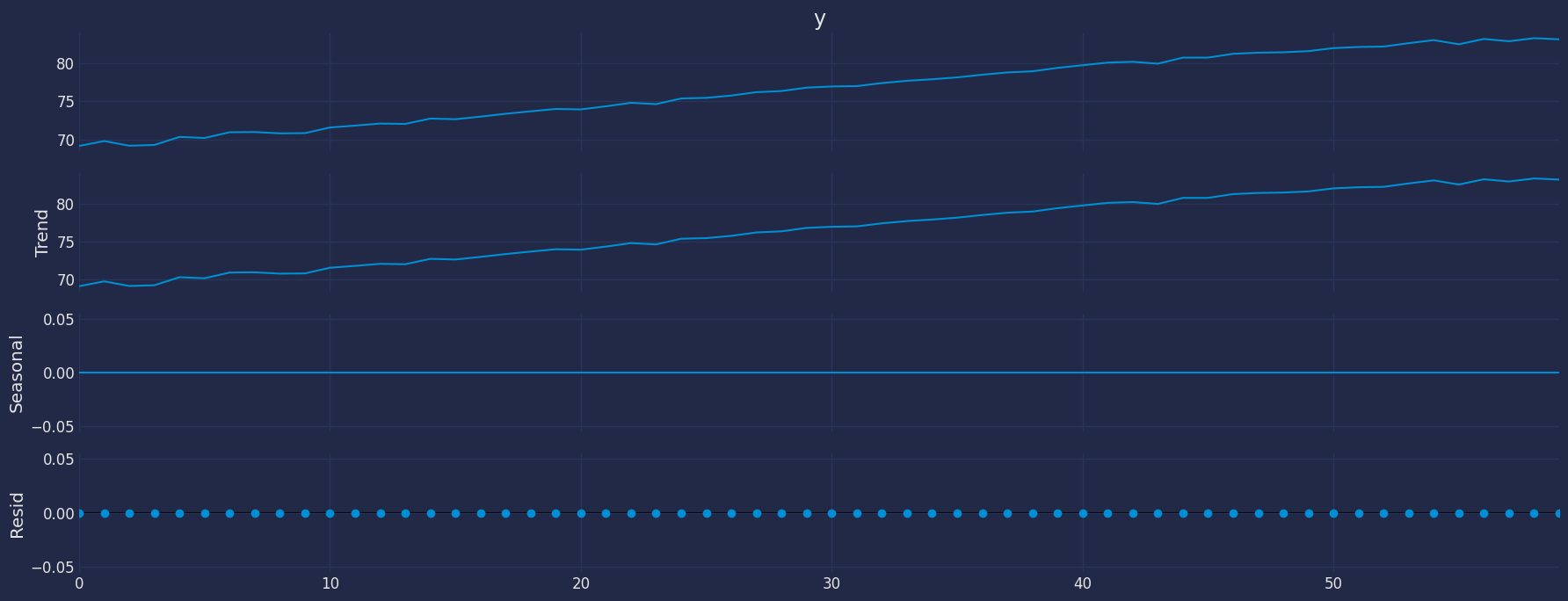
How to decompose a time series and why?
In time series analysis to forecast new values, it is very important to
know past data. More formally, we can say that it is very important to
know the patterns that values follow over time. There can be many
reasons that cause our forecast values to fall in the wrong direction.
Basically, a time series consists of four components. The variation of
those components causes the change in the pattern of the time series.
These components are:
* **Level:** This is the primary value that averages over time.
* **Trend:** The trend is the value that causes increasing or
decreasing patterns in a time series.
* **Seasonality:** This is a cyclical event that occurs in a time
series for a short time and causes short-term increasing or
decreasing patterns in a time series.
* **Residual/Noise:** These are the random variations in the time
series.
Combining these components over time leads to the formation of a time
series. Most time series consist of level and noise/residual and trend
or seasonality are optional values.
If seasonality and trend are part of the time series, then there will be
effects on the forecast value. As the pattern of the forecasted time
series may be different from the previous time series.
The combination of the components in time series can be of two types: \*
Additive \* multiplicative
### Additive time series
If the components of the time series are added to make the time series.
Then the time series is called the additive time series. By
visualization, we can say that the time series is additive if the
increasing or decreasing pattern of the time series is similar
throughout the series. The mathematical function of any additive time
series can be represented by:
$y(t) = level + Trend + seasonality + noise$
### Multiplicative time series
If the components of the time series are multiplicative together, then
the time series is called a multiplicative time series. For
visualization, if the time series is having exponential growth or
decline with time, then the time series can be considered as the
multiplicative time series. The mathematical function of the
multiplicative time series can be represented as.
$y(t) = Level * Trend * seasonality * Noise$
```python theme={null}
from statsmodels.tsa.seasonal import seasonal_decompose
```
```python theme={null}
decomposed=seasonal_decompose(df["y"], model = "add", period=1)
decomposed.plot()
plt.show()
```
### Seasonal Decomposed
How to decompose a time series and why?
In time series analysis to forecast new values, it is very important to
know past data. More formally, we can say that it is very important to
know the patterns that values follow over time. There can be many
reasons that cause our forecast values to fall in the wrong direction.
Basically, a time series consists of four components. The variation of
those components causes the change in the pattern of the time series.
These components are:
* **Level:** This is the primary value that averages over time.
* **Trend:** The trend is the value that causes increasing or
decreasing patterns in a time series.
* **Seasonality:** This is a cyclical event that occurs in a time
series for a short time and causes short-term increasing or
decreasing patterns in a time series.
* **Residual/Noise:** These are the random variations in the time
series.
Combining these components over time leads to the formation of a time
series. Most time series consist of level and noise/residual and trend
or seasonality are optional values.
If seasonality and trend are part of the time series, then there will be
effects on the forecast value. As the pattern of the forecasted time
series may be different from the previous time series.
The combination of the components in time series can be of two types: \*
Additive \* multiplicative
### Additive time series
If the components of the time series are added to make the time series.
Then the time series is called the additive time series. By
visualization, we can say that the time series is additive if the
increasing or decreasing pattern of the time series is similar
throughout the series. The mathematical function of any additive time
series can be represented by:
$y(t) = level + Trend + seasonality + noise$
### Multiplicative time series
If the components of the time series are multiplicative together, then
the time series is called a multiplicative time series. For
visualization, if the time series is having exponential growth or
decline with time, then the time series can be considered as the
multiplicative time series. The mathematical function of the
multiplicative time series can be represented as.
$y(t) = Level * Trend * seasonality * Noise$
```python theme={null}
from statsmodels.tsa.seasonal import seasonal_decompose
```
```python theme={null}
decomposed=seasonal_decompose(df["y"], model = "add", period=1)
decomposed.plot()
plt.show()
```
 ### The Augmented Dickey-Fuller Test
An Augmented Dickey-Fuller (ADF) test is a type of statistical test that
determines whether a unit root is present in time series data. Unit
roots can cause unpredictable results in time series analysis. A null
hypothesis is formed in the unit root test to determine how strongly
time series data is affected by a trend. By accepting the null
hypothesis, we accept the evidence that the time series data is not
stationary. By rejecting the null hypothesis or accepting the
alternative hypothesis, we accept the evidence that the time series data
is generated by a stationary process. This process is also known as
stationary trend. The values of the ADF test statistic are negative.
Lower ADF values indicate a stronger rejection of the null hypothesis.
Augmented Dickey-Fuller Test is a common statistical test used to test
whether a given time series is stationary or not. We can achieve this by
defining the null and alternate hypothesis.
Null Hypothesis: Time Series is non-stationary. It gives a
time-dependent trend. Alternate Hypothesis: Time Series is stationary.
In another term, the series doesn’t depend on time.
ADF or t Statistic \< critical values: Reject the null hypothesis, time
series is stationary. ADF or t Statistic > critical values: Failed to
reject the null hypothesis, time series is non-stationary.
```python theme={null}
from statsmodels.tsa.stattools import adfuller
```
```python theme={null}
def Augmented_Dickey_Fuller_Test_func(series , column_name):
print (f'Dickey-Fuller test results for columns: {column_name}')
dftest = adfuller(series, autolag='AIC')
dfoutput = pd.Series(dftest[0:4], index=['Test Statistic','p-value','No Lags Used','Number of observations used'])
for key,value in dftest[4].items():
dfoutput['Critical Value (%s)'%key] = value
print (dfoutput)
if dftest[1] <= 0.05:
print("Conclusion:====>")
print("Reject the null hypothesis")
print("The data is stationary")
else:
print("Conclusion:====>")
print("The null hypothesis cannot be rejected")
print("The data is not stationary")
```
```python theme={null}
Augmented_Dickey_Fuller_Test_func(df["y"],"Life expectancy")
```
```text theme={null}
Dickey-Fuller test results for columns: Life expectancy
Test Statistic -1.578590
p-value 0.494339
No Lags Used 2.000000
...
Critical Value (1%) -3.550670
Critical Value (5%) -2.913766
Critical Value (10%) -2.594624
Length: 7, dtype: float64
Conclusion:====>
The null hypothesis cannot be rejected
The data is not stationary
```
We can see in the result that we obtained the non-stationary series,
because the p-value is greater than 5%.
One of the objectives of applying the ADF test is to know if our series
is stationary, knowing the result of the ADF test, then we can determine
the next step. For our case, it can be seen from the previous result
that the time series is not stationary, so we will proceed to the next
step, which is to differentiate our time series.
We are going to create a copy of our data, with the objective of
investigating to find the stationarity in our time series.
Once we have made the copy of the time series, we are going to
differentiate the time series, and then we will use the augmented Dickey
Fuller test to investigate if our time series is stationary.
```python theme={null}
df1=df.copy()
df1['y_diff'] = df['y'].diff()
df1.dropna(inplace=True)
df1.head()
```
| | ds | y | unique\_id | y\_diff |
| - | ---------- | --------- | ---------- | --------- |
| 1 | 1961-01-01 | 69.760244 | 1 | 0.636341 |
| 2 | 1962-01-01 | 69.149756 | 1 | -0.610488 |
| 3 | 1963-01-01 | 69.248049 | 1 | 0.098293 |
| 4 | 1964-01-01 | 70.311707 | 1 | 1.063659 |
| 5 | 1965-01-01 | 70.171707 | 1 | -0.140000 |
Let’s apply the Dickey Fuller test again to find out if our time series
is already stationary.
```python theme={null}
Augmented_Dickey_Fuller_Test_func(df1["y_diff"],"Life expectancy")
```
```text theme={null}
Dickey-Fuller test results for columns: Life expectancy
Test Statistic -8.510100e+00
p-value 1.173776e-13
No Lags Used 1.000000e+00
...
Critical Value (1%) -3.550670e+00
Critical Value (5%) -2.913766e+00
Critical Value (10%) -2.594624e+00
Length: 7, dtype: float64
Conclusion:====>
Reject the null hypothesis
The data is stationary
```
We can observe in the previous result that now if our time series is
stationary, the p-value is less than 5%.
Now our time series is stationary, that is, we have only differentiated
1 time, therefore, the order of our parameter $d=1$.
```python theme={null}
from statsmodels.graphics.tsaplots import plot_acf, plot_pacf
import matplotlib.pyplot as plt
fig, axes = plt.subplots(2, 2, )
axes[0, 0].plot(df1["y"]); axes[0, 0].set_title('Original Series')
plot_acf(df1["y"], ax=axes[0, 1],lags=20)
axes[1, 0].plot(df1["y"].diff()); axes[1, 0].set_title('1st Order Differencing')
plot_acf(df1["y"].diff().dropna(), ax=axes[1, 1],lags=20)
plt.show()
```
### The Augmented Dickey-Fuller Test
An Augmented Dickey-Fuller (ADF) test is a type of statistical test that
determines whether a unit root is present in time series data. Unit
roots can cause unpredictable results in time series analysis. A null
hypothesis is formed in the unit root test to determine how strongly
time series data is affected by a trend. By accepting the null
hypothesis, we accept the evidence that the time series data is not
stationary. By rejecting the null hypothesis or accepting the
alternative hypothesis, we accept the evidence that the time series data
is generated by a stationary process. This process is also known as
stationary trend. The values of the ADF test statistic are negative.
Lower ADF values indicate a stronger rejection of the null hypothesis.
Augmented Dickey-Fuller Test is a common statistical test used to test
whether a given time series is stationary or not. We can achieve this by
defining the null and alternate hypothesis.
Null Hypothesis: Time Series is non-stationary. It gives a
time-dependent trend. Alternate Hypothesis: Time Series is stationary.
In another term, the series doesn’t depend on time.
ADF or t Statistic \< critical values: Reject the null hypothesis, time
series is stationary. ADF or t Statistic > critical values: Failed to
reject the null hypothesis, time series is non-stationary.
```python theme={null}
from statsmodels.tsa.stattools import adfuller
```
```python theme={null}
def Augmented_Dickey_Fuller_Test_func(series , column_name):
print (f'Dickey-Fuller test results for columns: {column_name}')
dftest = adfuller(series, autolag='AIC')
dfoutput = pd.Series(dftest[0:4], index=['Test Statistic','p-value','No Lags Used','Number of observations used'])
for key,value in dftest[4].items():
dfoutput['Critical Value (%s)'%key] = value
print (dfoutput)
if dftest[1] <= 0.05:
print("Conclusion:====>")
print("Reject the null hypothesis")
print("The data is stationary")
else:
print("Conclusion:====>")
print("The null hypothesis cannot be rejected")
print("The data is not stationary")
```
```python theme={null}
Augmented_Dickey_Fuller_Test_func(df["y"],"Life expectancy")
```
```text theme={null}
Dickey-Fuller test results for columns: Life expectancy
Test Statistic -1.578590
p-value 0.494339
No Lags Used 2.000000
...
Critical Value (1%) -3.550670
Critical Value (5%) -2.913766
Critical Value (10%) -2.594624
Length: 7, dtype: float64
Conclusion:====>
The null hypothesis cannot be rejected
The data is not stationary
```
We can see in the result that we obtained the non-stationary series,
because the p-value is greater than 5%.
One of the objectives of applying the ADF test is to know if our series
is stationary, knowing the result of the ADF test, then we can determine
the next step. For our case, it can be seen from the previous result
that the time series is not stationary, so we will proceed to the next
step, which is to differentiate our time series.
We are going to create a copy of our data, with the objective of
investigating to find the stationarity in our time series.
Once we have made the copy of the time series, we are going to
differentiate the time series, and then we will use the augmented Dickey
Fuller test to investigate if our time series is stationary.
```python theme={null}
df1=df.copy()
df1['y_diff'] = df['y'].diff()
df1.dropna(inplace=True)
df1.head()
```
| | ds | y | unique\_id | y\_diff |
| - | ---------- | --------- | ---------- | --------- |
| 1 | 1961-01-01 | 69.760244 | 1 | 0.636341 |
| 2 | 1962-01-01 | 69.149756 | 1 | -0.610488 |
| 3 | 1963-01-01 | 69.248049 | 1 | 0.098293 |
| 4 | 1964-01-01 | 70.311707 | 1 | 1.063659 |
| 5 | 1965-01-01 | 70.171707 | 1 | -0.140000 |
Let’s apply the Dickey Fuller test again to find out if our time series
is already stationary.
```python theme={null}
Augmented_Dickey_Fuller_Test_func(df1["y_diff"],"Life expectancy")
```
```text theme={null}
Dickey-Fuller test results for columns: Life expectancy
Test Statistic -8.510100e+00
p-value 1.173776e-13
No Lags Used 1.000000e+00
...
Critical Value (1%) -3.550670e+00
Critical Value (5%) -2.913766e+00
Critical Value (10%) -2.594624e+00
Length: 7, dtype: float64
Conclusion:====>
Reject the null hypothesis
The data is stationary
```
We can observe in the previous result that now if our time series is
stationary, the p-value is less than 5%.
Now our time series is stationary, that is, we have only differentiated
1 time, therefore, the order of our parameter $d=1$.
```python theme={null}
from statsmodels.graphics.tsaplots import plot_acf, plot_pacf
import matplotlib.pyplot as plt
fig, axes = plt.subplots(2, 2, )
axes[0, 0].plot(df1["y"]); axes[0, 0].set_title('Original Series')
plot_acf(df1["y"], ax=axes[0, 1],lags=20)
axes[1, 0].plot(df1["y"].diff()); axes[1, 0].set_title('1st Order Differencing')
plot_acf(df1["y"].diff().dropna(), ax=axes[1, 1],lags=20)
plt.show()
```
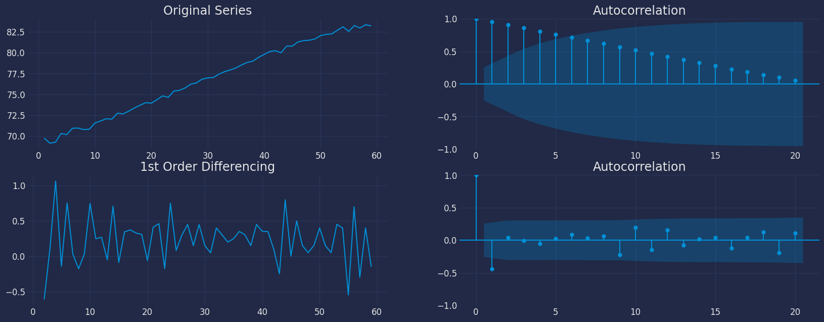 * For the above data, we can see that the time series reaches
stationarity with one orders of differencing.
## How to find the order of the AR term (p)
* The next step is to identify if the model needs any AR terms. We
will find out the required number of AR terms by inspecting the
**Partial Autocorrelation (PACF) plot**.
* **Partial autocorrelation** can be imagined as the correlation
between the series and its lag, after excluding the contributions
from the intermediate lags. So, PACF sort of conveys the pure
correlation between a lag and the series. This way, we will know if
that lag is needed in the AR term or not.
* Partial autocorrelation of lag (k) of a series is the coefficient of
that lag in the autoregression equation of $Y$.
$Yt = \alpha0 + \alpha1 Y{t-1} + \alpha2 Y{t-2} + \alpha3 Y{t-3}$
* That is, suppose, if $Y_t$ is the current series and $Y_{t-1}$ is
the lag 1 of $Y$, then the partial autocorrelation of lag 3
$(Y_{t-3})$ is the coefficient $\alpha_3$ of $Y_{t-3}$ in the above
equation.
* Now, we should find the number of AR terms. Any autocorrelation in a
stationarized series can be rectified by adding enough AR terms. So,
we initially take the order of AR term to be equal to as many lags
that crosses the significance limit in the PACF plot.
```python theme={null}
fig, axes = plt.subplots(1, 2)
axes[0].plot(df1["y"].diff()); axes[0].set_title('1st Differencing')
axes[1].set(ylim=(0,5))
plot_pacf(df1["y"].diff().dropna(), ax=axes[1],lags=20)
plt.show()
```
* For the above data, we can see that the time series reaches
stationarity with one orders of differencing.
## How to find the order of the AR term (p)
* The next step is to identify if the model needs any AR terms. We
will find out the required number of AR terms by inspecting the
**Partial Autocorrelation (PACF) plot**.
* **Partial autocorrelation** can be imagined as the correlation
between the series and its lag, after excluding the contributions
from the intermediate lags. So, PACF sort of conveys the pure
correlation between a lag and the series. This way, we will know if
that lag is needed in the AR term or not.
* Partial autocorrelation of lag (k) of a series is the coefficient of
that lag in the autoregression equation of $Y$.
$Yt = \alpha0 + \alpha1 Y{t-1} + \alpha2 Y{t-2} + \alpha3 Y{t-3}$
* That is, suppose, if $Y_t$ is the current series and $Y_{t-1}$ is
the lag 1 of $Y$, then the partial autocorrelation of lag 3
$(Y_{t-3})$ is the coefficient $\alpha_3$ of $Y_{t-3}$ in the above
equation.
* Now, we should find the number of AR terms. Any autocorrelation in a
stationarized series can be rectified by adding enough AR terms. So,
we initially take the order of AR term to be equal to as many lags
that crosses the significance limit in the PACF plot.
```python theme={null}
fig, axes = plt.subplots(1, 2)
axes[0].plot(df1["y"].diff()); axes[0].set_title('1st Differencing')
axes[1].set(ylim=(0,5))
plot_pacf(df1["y"].diff().dropna(), ax=axes[1],lags=20)
plt.show()
```
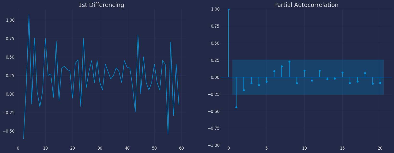 * We can see that the PACF lag 1 is quite significant since it is well
above the significance line. So, we will fix the value of p as 1.
## How to find the order of the MA term (q)
* Just like how we looked at the PACF plot for the number of AR terms,
we will look at the ACF plot for the number of MA terms. An MA term
is technically, the error of the lagged forecast.
* The ACF tells how many MA terms are required to remove any
autocorrelation in the stationarized series.
* Let’s see the autocorrelation plot of the differenced series.
```python theme={null}
from statsmodels.graphics.tsaplots import plot_acf
fig, axes = plt.subplots(1, 2)
axes[0].plot(df1["y"].diff()); axes[0].set_title('1st Differencing')
axes[1].set(ylim=(0,1.2))
plot_acf(df["y"].diff().dropna(), ax=axes[1], lags=20)
plt.show()
```
* We can see that the PACF lag 1 is quite significant since it is well
above the significance line. So, we will fix the value of p as 1.
## How to find the order of the MA term (q)
* Just like how we looked at the PACF plot for the number of AR terms,
we will look at the ACF plot for the number of MA terms. An MA term
is technically, the error of the lagged forecast.
* The ACF tells how many MA terms are required to remove any
autocorrelation in the stationarized series.
* Let’s see the autocorrelation plot of the differenced series.
```python theme={null}
from statsmodels.graphics.tsaplots import plot_acf
fig, axes = plt.subplots(1, 2)
axes[0].plot(df1["y"].diff()); axes[0].set_title('1st Differencing')
axes[1].set(ylim=(0,1.2))
plot_acf(df["y"].diff().dropna(), ax=axes[1], lags=20)
plt.show()
```
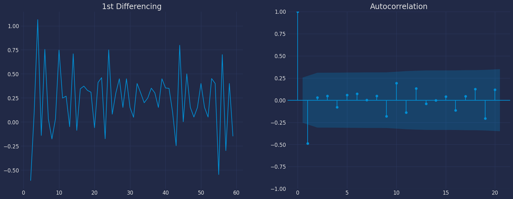 * We can see that couple of lags are well above the significance line.
So, we will fix q as 1. If there is any doubt, we will go with the
simpler model that sufficiently explains the Y.
## How to handle if a time series is slightly under or over differenced
* It may happen that the time series is slightly under differenced.
Differencing it one more time makes it slightly over-differenced.
* If the series is slightly under differenced, adding one or more
additional AR terms usually makes it up. Likewise, if it is slightly
over-differenced, we will try adding an additional MA term.
## Implementation of ARIMA with StatsForecast
Now, we have determined the values of p, d and q. We have everything
needed to fit the ARIMA model. We will use the ARIMA() implementation in
the `statsforecast` package.
The parameters found are: \* For the autoregressive model, $p=1$ \* for
the moving average model $q=1$ \* and for the stationarity of the model
with a differential with an order $d=1$
Therefore, the model that we are going to test is the ARIMA(1,1,1)
model.
```python theme={null}
from statsforecast import StatsForecast
from statsforecast.models import ARIMA
```
### Instantiate the model
```python theme={null}
sf = StatsForecast(models=[ARIMA(order=(1, 1, 1))], freq='YS')
```
### Fit the Model
```python theme={null}
sf.fit(df)
```
```text theme={null}
StatsForecast(models=[ARIMA])
```
### Making the predictions
```python theme={null}
y_hat = sf.predict(h=6)
y_hat
```
| | unique\_id | ds | ARIMA |
| - | ---------- | ---------- | --------- |
| 0 | 1 | 2020-01-01 | 83.206903 |
| 1 | 1 | 2021-01-01 | 83.203508 |
| 2 | 1 | 2022-01-01 | 83.204742 |
| 3 | 1 | 2023-01-01 | 83.204293 |
| 4 | 1 | 2024-01-01 | 83.204456 |
| 5 | 1 | 2025-01-01 | 83.204397 |
We can make the predictions by adding the confidence interval, for
example with 95%.
```python theme={null}
y_hat2 = sf.predict(h=6, level=[95])
y_hat2
```
| | unique\_id | ds | ARIMA | ARIMA-lo-95 | ARIMA-hi-95 |
| - | ---------- | ---------- | --------- | ----------- | ----------- |
| 0 | 1 | 2020-01-01 | 83.206903 | 82.412336 | 84.001469 |
| 1 | 1 | 2021-01-01 | 83.203508 | 82.094625 | 84.312391 |
| 2 | 1 | 2022-01-01 | 83.204742 | 81.848344 | 84.561139 |
| 3 | 1 | 2023-01-01 | 83.204293 | 81.640430 | 84.768156 |
| 4 | 1 | 2024-01-01 | 83.204456 | 81.457145 | 84.951767 |
| 5 | 1 | 2025-01-01 | 83.204397 | 81.291297 | 85.117497 |
### forecast method
Memory efficient predictions.
This method avoids memory burden due from object storage. It is
analogous to fit\_predict without storing information. It assumes you
know the forecast horizon in advance.
```python theme={null}
Y_hat_df = sf.forecast(df=df, h=6, level=[95])
Y_hat_df
```
| | unique\_id | ds | ARIMA | ARIMA-lo-95 | ARIMA-hi-95 |
| - | ---------- | ---------- | --------- | ----------- | ----------- |
| 0 | 1 | 2020-01-01 | 83.206903 | 82.412336 | 84.001469 |
| 1 | 1 | 2021-01-01 | 83.203508 | 82.094625 | 84.312391 |
| 2 | 1 | 2022-01-01 | 83.204742 | 81.848344 | 84.561139 |
| 3 | 1 | 2023-01-01 | 83.204293 | 81.640430 | 84.768156 |
| 4 | 1 | 2024-01-01 | 83.204456 | 81.457145 | 84.951767 |
| 5 | 1 | 2025-01-01 | 83.204397 | 81.291297 | 85.117497 |
Once the predictions have been generated we can perform a visualization
to see the generated behavior of our model.
```python theme={null}
sf.plot(df, Y_hat_df, level=[95])
```
* We can see that couple of lags are well above the significance line.
So, we will fix q as 1. If there is any doubt, we will go with the
simpler model that sufficiently explains the Y.
## How to handle if a time series is slightly under or over differenced
* It may happen that the time series is slightly under differenced.
Differencing it one more time makes it slightly over-differenced.
* If the series is slightly under differenced, adding one or more
additional AR terms usually makes it up. Likewise, if it is slightly
over-differenced, we will try adding an additional MA term.
## Implementation of ARIMA with StatsForecast
Now, we have determined the values of p, d and q. We have everything
needed to fit the ARIMA model. We will use the ARIMA() implementation in
the `statsforecast` package.
The parameters found are: \* For the autoregressive model, $p=1$ \* for
the moving average model $q=1$ \* and for the stationarity of the model
with a differential with an order $d=1$
Therefore, the model that we are going to test is the ARIMA(1,1,1)
model.
```python theme={null}
from statsforecast import StatsForecast
from statsforecast.models import ARIMA
```
### Instantiate the model
```python theme={null}
sf = StatsForecast(models=[ARIMA(order=(1, 1, 1))], freq='YS')
```
### Fit the Model
```python theme={null}
sf.fit(df)
```
```text theme={null}
StatsForecast(models=[ARIMA])
```
### Making the predictions
```python theme={null}
y_hat = sf.predict(h=6)
y_hat
```
| | unique\_id | ds | ARIMA |
| - | ---------- | ---------- | --------- |
| 0 | 1 | 2020-01-01 | 83.206903 |
| 1 | 1 | 2021-01-01 | 83.203508 |
| 2 | 1 | 2022-01-01 | 83.204742 |
| 3 | 1 | 2023-01-01 | 83.204293 |
| 4 | 1 | 2024-01-01 | 83.204456 |
| 5 | 1 | 2025-01-01 | 83.204397 |
We can make the predictions by adding the confidence interval, for
example with 95%.
```python theme={null}
y_hat2 = sf.predict(h=6, level=[95])
y_hat2
```
| | unique\_id | ds | ARIMA | ARIMA-lo-95 | ARIMA-hi-95 |
| - | ---------- | ---------- | --------- | ----------- | ----------- |
| 0 | 1 | 2020-01-01 | 83.206903 | 82.412336 | 84.001469 |
| 1 | 1 | 2021-01-01 | 83.203508 | 82.094625 | 84.312391 |
| 2 | 1 | 2022-01-01 | 83.204742 | 81.848344 | 84.561139 |
| 3 | 1 | 2023-01-01 | 83.204293 | 81.640430 | 84.768156 |
| 4 | 1 | 2024-01-01 | 83.204456 | 81.457145 | 84.951767 |
| 5 | 1 | 2025-01-01 | 83.204397 | 81.291297 | 85.117497 |
### forecast method
Memory efficient predictions.
This method avoids memory burden due from object storage. It is
analogous to fit\_predict without storing information. It assumes you
know the forecast horizon in advance.
```python theme={null}
Y_hat_df = sf.forecast(df=df, h=6, level=[95])
Y_hat_df
```
| | unique\_id | ds | ARIMA | ARIMA-lo-95 | ARIMA-hi-95 |
| - | ---------- | ---------- | --------- | ----------- | ----------- |
| 0 | 1 | 2020-01-01 | 83.206903 | 82.412336 | 84.001469 |
| 1 | 1 | 2021-01-01 | 83.203508 | 82.094625 | 84.312391 |
| 2 | 1 | 2022-01-01 | 83.204742 | 81.848344 | 84.561139 |
| 3 | 1 | 2023-01-01 | 83.204293 | 81.640430 | 84.768156 |
| 4 | 1 | 2024-01-01 | 83.204456 | 81.457145 | 84.951767 |
| 5 | 1 | 2025-01-01 | 83.204397 | 81.291297 | 85.117497 |
Once the predictions have been generated we can perform a visualization
to see the generated behavior of our model.
```python theme={null}
sf.plot(df, Y_hat_df, level=[95])
```
 ## Model Evaluation
The commonly used accuracy metrics to judge forecasts are:
1. Mean Absolute Percentage Error (MAPE)
2. Mean Error (ME)
3. Mean Absolute Error (MAE)
4. Mean Percentage Error (MPE)
5. Root Mean Squared Error (RMSE)
6. Correlation between the Actual and the Forecast (corr)
```python theme={null}
Y_train_df = df[df.ds<='2013-01-01']
Y_test_df = df[df.ds>'2013-01-01']
Y_train_df.shape, Y_test_df.shape
```
```text theme={null}
((54, 3), (6, 3))
```
```python theme={null}
Y_hat_df = sf.forecast(df=Y_train_df, h=len(Y_test_df))
```
```python theme={null}
import utilsforecast.losses as ufl
from utilsforecast.evaluation import evaluate
```
```python theme={null}
evaluate(
Y_test_df.merge(Y_hat_df),
metrics=[ufl.mse, ufl.mae, ufl.rmse, ufl.mape],
)
```
| | unique\_id | metric | ARIMA |
| - | ---------- | ------ | -------- |
| 0 | 1 | mse | 0.184000 |
| 1 | 1 | mae | 0.397932 |
| 2 | 1 | rmse | 0.428952 |
| 3 | 1 | mape | 0.004785 |
## References
1. [Nixtla ARIMA API](../../src/core/models.html#arima)
2. [Rob J. Hyndman and George Athanasopoulos (2018). “Forecasting
Principles and Practice (3rd
ed)”](https://otexts.com/fpp3/tscv.html).
## Model Evaluation
The commonly used accuracy metrics to judge forecasts are:
1. Mean Absolute Percentage Error (MAPE)
2. Mean Error (ME)
3. Mean Absolute Error (MAE)
4. Mean Percentage Error (MPE)
5. Root Mean Squared Error (RMSE)
6. Correlation between the Actual and the Forecast (corr)
```python theme={null}
Y_train_df = df[df.ds<='2013-01-01']
Y_test_df = df[df.ds>'2013-01-01']
Y_train_df.shape, Y_test_df.shape
```
```text theme={null}
((54, 3), (6, 3))
```
```python theme={null}
Y_hat_df = sf.forecast(df=Y_train_df, h=len(Y_test_df))
```
```python theme={null}
import utilsforecast.losses as ufl
from utilsforecast.evaluation import evaluate
```
```python theme={null}
evaluate(
Y_test_df.merge(Y_hat_df),
metrics=[ufl.mse, ufl.mae, ufl.rmse, ufl.mape],
)
```
| | unique\_id | metric | ARIMA |
| - | ---------- | ------ | -------- |
| 0 | 1 | mse | 0.184000 |
| 1 | 1 | mae | 0.397932 |
| 2 | 1 | rmse | 0.428952 |
| 3 | 1 | mape | 0.004785 |
## References
1. [Nixtla ARIMA API](../../src/core/models.html#arima)
2. [Rob J. Hyndman and George Athanasopoulos (2018). “Forecasting
Principles and Practice (3rd
ed)”](https://otexts.com/fpp3/tscv.html).