> ## Documentation Index
> Fetch the complete documentation index at: https://nixtlaverse.nixtla.io/llms.txt
> Use this file to discover all available pages before exploring further.
# ARCH Model
> Step-by-step guide on using the `ARCH Model` with `Statsforecast`.
In this walkthrough, we will become familiar with the main
`StatsForecast` class and some relevant methods such as
`StatsForecast.plot`, `StatsForecast.forecast` and
`StatsForecast.cross_validation`.
The text in this article is largely taken from [Changquan Huang • Alla
Petukhina. Springer series (2022). Applied Time Series Analysis and
Forecasting with
Python.](https://link.springer.com/book/10.1007/978-3-031-13584-2)
## Table of Contents
* [Introduction](#introduction)
* [ARCH Models](#model)
* [Loading libraries and data](#loading)
* [Explore data with the plot method](#plotting)
* [Split the data into training and testing](#splitting)
* [Implementation of ARCH with StatsForecast](#implementation)
* [Cross-validation](#cross_validate)
* [Model evaluation](#evaluate)
* [References](#references)
## Introduction
Financial time series analysis has been one of the hottest research
topics in the recent decades. In this guide, we illustrate the stylized
facts of financial time series by real financial data. To characterize
these facts, new models different from the Box- Jenkins ones are needed.
And for this reason, ARCH models were firstly proposed by R. F. Engle in
1982 and have been extended by a great number of scholars since then. We
also demonstrate how to use Python and its libraries to implement
`ARCH`.
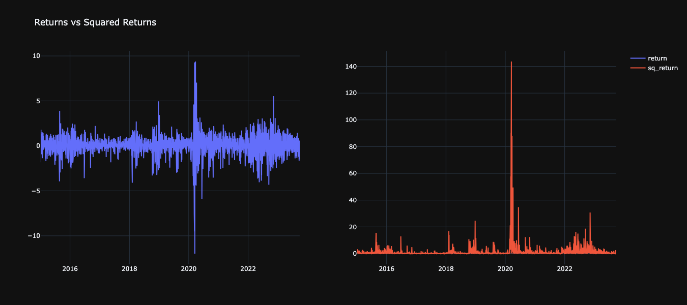
As we have known, there are lot of time series that possess the ARCH
effect, that is, although the (modeling residual) series is white noise,
its squared series may be autocorrelated. What is more, in practice, a
large number of financial time series are found having this property so
that the ARCH effect has become one of the stylized facts from financial
time series.
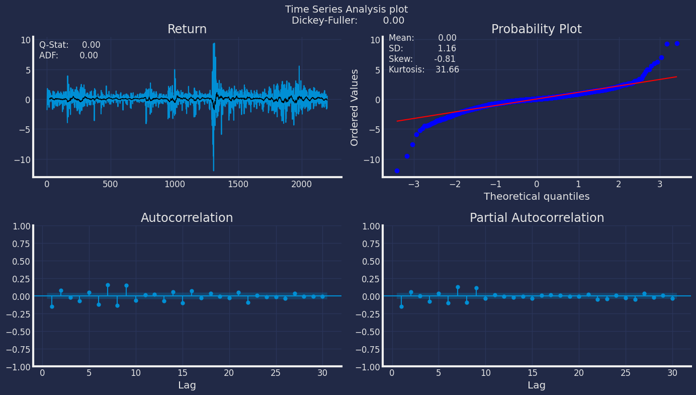
### Stylized Facts of Financial Time Series
Now we briefly list and describe several important stylized facts
(features) of financial return series:
* **Fat (heavy) tails:** The distribution density function of returns
often has fatter (heavier) tails than the tails of the corresponding
normal distribution density.
* **ARCH effect:** Although the return series can often be seen as a
white noise, its squared (and absolute) series may usually be
autocorrelated, and these autocorrelations are hardly negative.
* **Volatility clustering:** Large changes in returns tend to cluster
in time, and small changes tend to be followed by small changes.
* **Asymmetry:** As we have know , the distribution of asset returns
is slightly negatively skewed. One possible explanation could be
that traders react more strongly to unfavorable information than
favorable information.
## Definition of ARCH Models
Specifically, we give the definition of the ARCH model as follows.
**Definition 1.** An $\text{ARCH(p)}$ model with order $p≥1$ is of the
form
$$
\begin{equation}
\left\{
\begin{array}{ll}
X_t =\sigma_t \varepsilon_t \\
\sigma_{t}^2 =\omega+ \alpha_1 X_{t-1}^2 + \alpha_2 X_{t-2}^2 + \cdots+ \alpha_p X_{t-p}^2 \\
\end{array}
\right.
\end{equation}
$$
where $\omega ≥ 0, \alpha_i ≥ 0$, and $\alpha_p > 0$ are constants,
$\varepsilon_t \sim iid(0, 1)$, and $\varepsilon_t$ is independent of
$\{X_k;k ≤ t − 1 \}$. A stochastic process $X_t$ is called an $ARCH(p)$
process if it satisfies Eq. (1).
By Definition 1, $\sigma_{t}^2$ (and $\sigma_t$ ) is independent of
$\varepsilon_t$ . Besides, usually it is further assumed that
$\varepsilon_t \sim N(0, 1)$. Sometimes, however, we need to further
suppose that $\varepsilon_t$ follows a standardized (skew) Student’s T
distribution or a generalized error distribution in order to capture
more features of a financial time series.
Let $\mathscr{F}_s$ denote the information set generated by
$\{X_k;k ≤ s \}$, namely, the sigma field $\sigma(X_k;k ≤ s)$. It is
easy to see that $\mathscr{F}_s$ is independent of $\varepsilon_t$ for
any $s 0$, in light of the properties of the conditional
mathematical expectation and by (2), we have that
$E(X_{t+h} X_t) = E(E(X_{t+h} X_t|\mathscr{F}_{t+h-1})) = E(X_t E(X_{t+h}|\mathscr{F}_{t+h-1})) = 0.$
In conclusion, if $0 < \alpha_1 < 1$, we have that:
* Any $\text{ARCH}(1)$ process $\{X_t \}$ defined by Eqs.(3) follows a
white noise $WN(0, \omega/(1 − \alpha_1))$ .
* Since $X_{t}^2$ is an $\text{AR}(1)$ process defined by (4),
$\text{Corr}(X_{t}^2,X_{t+h}^2) = \alpha_{1}^{|h|} > 0$, which
reveals the ARCH effect.
* It is clear that $E(\eta_t|\mathscr{F}_s)=0$ for any $t>s$,and with
Eq.(4),for any $k>1$:
$Var(X_{t+k} |\mathscr{F}_t ) = E(X_{t+K}^2 |\mathscr{F}_t)$
$= E(\omega + \alpha_1 X_{t+k-1}+ \eta_{t+k}|\mathscr{F}_t )$
$= \omega + \alpha_1 Var(X_{t+k−1}|\mathscr{F}_t),$
which reflects the volatility clustering, that is, large (small)
volatility is followed by large (small) one.
In addition, we are able to prove that Xt defined by Eq. (3) has heavier
tails than the corresponding normal distribution. At last, note that
these properties of the ARCH(1) model can be generalized to ARCH(p)
models.
### Advantages and disadvantages of the Autoregressive Conditional Heteroskedasticity (ARCH) model:
| Advantages | Disadvantages |
| --------------------------------------------------------------------------------------------------------------------------------------------------- | ----------------------------------------------------------------------------------------------------------------------------------------------------------------- |
| - The ARCH model is useful for modeling volatility in financial time series, which is important for investment decision making and risk management. | - The ARCH model assumes that the forecast errors are independent and identically distributed, which may not be realistic in some cases. |
| - The ARCH model takes heteroscedasticity into account, which means that it can model time series with variances that change over time. | - The ARCH model can be difficult to fit to data with many parameters, which may require large amounts of data or advanced estimation techniques. |
| - The ARCH model is relatively easy to use and can be implemented with standard econometrics software. | - The ARCH model does not take into account the possible relationship between the mean and the variance of the time series, which may be important in some cases. |
Note:
The ARCH model is a useful tool for modeling volatility in financial
time series, but like any econometric model, it has limitations and
should be used with caution depending on the specific characteristics of
the data being modeled.
### Autoregressive Conditional Heteroskedasticity (ARCH) Applications
* **Finance** - The ARCH model is widely used in finance to model
volatility in financial time series, such as stock prices, exchange
rates, interest rates, etc.
* **Economics** - The ARCH model can be used to model volatility in
economic data, such as GDP, inflation, unemployment, among others.
* **Engineering** - The ARCH model can be used in engineering to model
volatility in data related to energy, climate, pollution, industrial
production, among others.
* **Social Sciences** - The ARCH model can be used in the social
sciences to model volatility in data related to demography, health,
education, among others.
* **Biology** - The ARCH model can be used in biology to model
volatility in data related to evolution, genetics, epidemiology,
among others.
## Loading libraries and data
> **Tip**
>
> Statsforecast will be needed. To install, see
> [instructions](../getting-started/installation.html).
Next, we import plotting libraries and configure the plotting style.
```python theme={null}
import matplotlib.pyplot as plt
from statsmodels.graphics.tsaplots import plot_acf
from statsmodels.graphics.tsaplots import plot_pacf
plt.style.use('fivethirtyeight')
plt.rcParams['lines.linewidth'] = 1.5
dark_style = {
'figure.facecolor': '#212946',
'axes.facecolor': '#212946',
'savefig.facecolor':'#212946',
'axes.grid': True,
'axes.grid.which': 'both',
'axes.spines.left': False,
'axes.spines.right': False,
'axes.spines.top': False,
'axes.spines.bottom': False,
'grid.color': '#2A3459',
'grid.linewidth': '1',
'text.color': '0.9',
'axes.labelcolor': '0.9',
'xtick.color': '0.9',
'ytick.color': '0.9',
'font.size': 12 }
plt.rcParams.update(dark_style)
from pylab import rcParams
rcParams['figure.figsize'] = (18,7)
```
### Read Data
Let’s pull the S\&P500 stock data from the Yahoo Finance site.
```python theme={null}
import datetime
import pandas as pd
import time
import yfinance as yf
ticker = '^GSPC'
period1 = datetime.datetime(2015, 1, 1)
period2 = datetime.datetime(2023, 9, 22)
interval = '1d' # 1d, 1m
SP_500 = yf.download(ticker, start=period1, end=period2, interval=interval, progress=False)
SP_500 = SP_500.reset_index()
SP_500.head()
```
| Price | Date | Adj Close | Close | High | Low | Open | Volume |
| ------ | ------------------------- | ----------- | ----------- | ----------- | ----------- | ----------- | ---------- |
| Ticker | | ^GSPC | ^GSPC | ^GSPC | ^GSPC | ^GSPC | ^GSPC |
| 0 | 2015-01-02 00:00:00+00:00 | 2058.199951 | 2058.199951 | 2072.360107 | 2046.040039 | 2058.899902 | 2708700000 |
| 1 | 2015-01-05 00:00:00+00:00 | 2020.579956 | 2020.579956 | 2054.439941 | 2017.339966 | 2054.439941 | 3799120000 |
| 2 | 2015-01-06 00:00:00+00:00 | 2002.609985 | 2002.609985 | 2030.250000 | 1992.439941 | 2022.150024 | 4460110000 |
| 3 | 2015-01-07 00:00:00+00:00 | 2025.900024 | 2025.900024 | 2029.609985 | 2005.550049 | 2005.550049 | 3805480000 |
| 4 | 2015-01-08 00:00:00+00:00 | 2062.139893 | 2062.139893 | 2064.080078 | 2030.609985 | 2030.609985 | 3934010000 |
```python theme={null}
df=SP_500[["Date","Close"]].copy()
```
The input to StatsForecast is always a data frame in long format with
three columns: unique\_id, ds and y:
* The `unique_id` (string, int or category) represents an identifier
for the series.
* The `ds` (datestamp) column should be of a format expected by
Pandas, ideally YYYY-MM-DD for a date or YYYY-MM-DD HH:MM:SS for a
timestamp.
* The `y` (numeric) represents the measurement we wish to forecast.
```python theme={null}
df["unique_id"]="1"
df.columns=["ds", "y", "unique_id"]
df.head()
```
| | ds | y | unique\_id |
| - | ------------------------- | ----------- | ---------- |
| 0 | 2015-01-02 00:00:00+00:00 | 2058.199951 | 1 |
| 1 | 2015-01-05 00:00:00+00:00 | 2020.579956 | 1 |
| 2 | 2015-01-06 00:00:00+00:00 | 2002.609985 | 1 |
| 3 | 2015-01-07 00:00:00+00:00 | 2025.900024 | 1 |
| 4 | 2015-01-08 00:00:00+00:00 | 2062.139893 | 1 |
```python theme={null}
print(df.dtypes)
```
```text theme={null}
ds datetime64[ns]
y float64
unique_id object
dtype: object
```
## Explore data with the plot method
Plot a series using the plot method from the StatsForecast class. This
method prints a random series from the dataset and is useful for basic
EDA.
```python theme={null}
from statsforecast import StatsForecast
StatsForecast.plot(df)
```
 ### The Augmented Dickey-Fuller Test
An Augmented Dickey-Fuller (ADF) test is a type of statistical test that
determines whether a unit root is present in time series data. Unit
roots can cause unpredictable results in time series analysis. A null
hypothesis is formed in the unit root test to determine how strongly
time series data is affected by a trend. By accepting the null
hypothesis, we accept the evidence that the time series data is not
stationary. By rejecting the null hypothesis or accepting the
alternative hypothesis, we accept the evidence that the time series data
is generated by a stationary process. This process is also known as
stationary trend. The values of the ADF test statistic are negative.
Lower ADF values indicate a stronger rejection of the null hypothesis.
Augmented Dickey-Fuller Test is a common statistical test used to test
whether a given time series is stationary or not. We can achieve this by
defining the null and alternate hypothesis.
Null Hypothesis: Time Series is non-stationary. It gives a
time-dependent trend. Alternate Hypothesis: Time Series is stationary.
In another term, the series doesn’t depend on time.
ADF or t Statistic \< critical values: Reject the null hypothesis, time
series is stationary. ADF or t Statistic > critical values: Failed to
reject the null hypothesis, time series is non-stationary.
Let’s check if our series that we are analyzing is a stationary series.
Let’s create a function to check, using the `Dickey Fuller` test
```python theme={null}
from statsmodels.tsa.stattools import adfuller
def Augmented_Dickey_Fuller_Test_func(series , column_name):
print (f'Dickey-Fuller test results for columns: {column_name}')
dftest = adfuller(series, autolag='AIC')
dfoutput = pd.Series(dftest[0:4], index=['Test Statistic','p-value','No Lags Used','Number of observations used'])
for key,value in dftest[4].items():
dfoutput['Critical Value (%s)'%key] = value
print (dfoutput)
if dftest[1] <= 0.05:
print("Conclusion:====>")
print("Reject the null hypothesis")
print("The data is stationary")
else:
print("Conclusion:====>")
print("The null hypothesis cannot be rejected")
print("The data is not stationary")
```
```python theme={null}
Augmented_Dickey_Fuller_Test_func(df["y"],'S&P500')
```
```text theme={null}
Dickey-Fuller test results for columns: S&P500
Test Statistic -0.814971
p-value 0.814685
No Lags Used 10.000000
...
Critical Value (1%) -3.433341
Critical Value (5%) -2.862861
Critical Value (10%) -2.567473
Length: 7, dtype: float64
Conclusion:====>
The null hypothesis cannot be rejected
The data is not stationary
```
In the previous result we can see that the `Augmented_Dickey_Fuller`
test gives us a `p-value` of 0.864700, which tells us that the null
hypothesis cannot be rejected, and on the other hand the data of our
series are not stationary.
We need to differentiate our time series, in order to convert the data
to stationary.
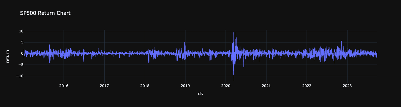
### Return Series
Since the 1970s, the financial industry has been very prosperous with
advancement of computer and Internet technology. Trade of financial
products (including various derivatives) generates a huge amount of data
which form financial time series. For finance, the return on a financial
product is most interesting, and so our attention focuses on the return
series. If $P_t$ is the closing price at time t for a certain financial
product, then the return on this product is
$X_t = \frac{(P_t − P_{t−1})}{P_{t−1}} ≈ log(P_t ) − log(P_{t−1}).$
It is return series $\{X_t \}$ that have been much independently
studied. And important stylized features which are common across many
instruments, markets, and time periods have been summarized. Note that
if you purchase the financial product, then it becomes your asset, and
its returns become your asset returns. Now let us look at the following
examples.
We can estimate the series of returns using the
[pandas](https://pandas.pydata.org/docs/reference/api/pandas.DataFrame.pct_change.html),
`DataFrame.pct_change()` function. The `pct_change()` function has a
periods parameter whose default value is 1. If you want to calculate a
30-day return, you must change the value to 30.
```python theme={null}
df['return'] = 100 * df["y"].pct_change()
df.dropna(inplace=True, how='any')
df.head()
```
| | ds | y | unique\_id | return |
| - | ------------------------- | ----------- | ---------- | --------- |
| 1 | 2015-01-05 00:00:00+00:00 | 2020.579956 | 1 | -1.827811 |
| 2 | 2015-01-06 00:00:00+00:00 | 2002.609985 | 1 | -0.889347 |
| 3 | 2015-01-07 00:00:00+00:00 | 2025.900024 | 1 | 1.162984 |
| 4 | 2015-01-08 00:00:00+00:00 | 2062.139893 | 1 | 1.788828 |
| 5 | 2015-01-09 00:00:00+00:00 | 2044.810059 | 1 | -0.840381 |
```python theme={null}
import plotly.express as px
fig = px.line(df, x=df["ds"], y="return",title="SP500 Return Chart",template = "plotly_dark")
fig.show()
```
### The Augmented Dickey-Fuller Test
An Augmented Dickey-Fuller (ADF) test is a type of statistical test that
determines whether a unit root is present in time series data. Unit
roots can cause unpredictable results in time series analysis. A null
hypothesis is formed in the unit root test to determine how strongly
time series data is affected by a trend. By accepting the null
hypothesis, we accept the evidence that the time series data is not
stationary. By rejecting the null hypothesis or accepting the
alternative hypothesis, we accept the evidence that the time series data
is generated by a stationary process. This process is also known as
stationary trend. The values of the ADF test statistic are negative.
Lower ADF values indicate a stronger rejection of the null hypothesis.
Augmented Dickey-Fuller Test is a common statistical test used to test
whether a given time series is stationary or not. We can achieve this by
defining the null and alternate hypothesis.
Null Hypothesis: Time Series is non-stationary. It gives a
time-dependent trend. Alternate Hypothesis: Time Series is stationary.
In another term, the series doesn’t depend on time.
ADF or t Statistic \< critical values: Reject the null hypothesis, time
series is stationary. ADF or t Statistic > critical values: Failed to
reject the null hypothesis, time series is non-stationary.
Let’s check if our series that we are analyzing is a stationary series.
Let’s create a function to check, using the `Dickey Fuller` test
```python theme={null}
from statsmodels.tsa.stattools import adfuller
def Augmented_Dickey_Fuller_Test_func(series , column_name):
print (f'Dickey-Fuller test results for columns: {column_name}')
dftest = adfuller(series, autolag='AIC')
dfoutput = pd.Series(dftest[0:4], index=['Test Statistic','p-value','No Lags Used','Number of observations used'])
for key,value in dftest[4].items():
dfoutput['Critical Value (%s)'%key] = value
print (dfoutput)
if dftest[1] <= 0.05:
print("Conclusion:====>")
print("Reject the null hypothesis")
print("The data is stationary")
else:
print("Conclusion:====>")
print("The null hypothesis cannot be rejected")
print("The data is not stationary")
```
```python theme={null}
Augmented_Dickey_Fuller_Test_func(df["y"],'S&P500')
```
```text theme={null}
Dickey-Fuller test results for columns: S&P500
Test Statistic -0.814971
p-value 0.814685
No Lags Used 10.000000
...
Critical Value (1%) -3.433341
Critical Value (5%) -2.862861
Critical Value (10%) -2.567473
Length: 7, dtype: float64
Conclusion:====>
The null hypothesis cannot be rejected
The data is not stationary
```
In the previous result we can see that the `Augmented_Dickey_Fuller`
test gives us a `p-value` of 0.864700, which tells us that the null
hypothesis cannot be rejected, and on the other hand the data of our
series are not stationary.
We need to differentiate our time series, in order to convert the data
to stationary.
### Return Series
Since the 1970s, the financial industry has been very prosperous with
advancement of computer and Internet technology. Trade of financial
products (including various derivatives) generates a huge amount of data
which form financial time series. For finance, the return on a financial
product is most interesting, and so our attention focuses on the return
series. If $P_t$ is the closing price at time t for a certain financial
product, then the return on this product is
$X_t = \frac{(P_t − P_{t−1})}{P_{t−1}} ≈ log(P_t ) − log(P_{t−1}).$
It is return series $\{X_t \}$ that have been much independently
studied. And important stylized features which are common across many
instruments, markets, and time periods have been summarized. Note that
if you purchase the financial product, then it becomes your asset, and
its returns become your asset returns. Now let us look at the following
examples.
We can estimate the series of returns using the
[pandas](https://pandas.pydata.org/docs/reference/api/pandas.DataFrame.pct_change.html),
`DataFrame.pct_change()` function. The `pct_change()` function has a
periods parameter whose default value is 1. If you want to calculate a
30-day return, you must change the value to 30.
```python theme={null}
df['return'] = 100 * df["y"].pct_change()
df.dropna(inplace=True, how='any')
df.head()
```
| | ds | y | unique\_id | return |
| - | ------------------------- | ----------- | ---------- | --------- |
| 1 | 2015-01-05 00:00:00+00:00 | 2020.579956 | 1 | -1.827811 |
| 2 | 2015-01-06 00:00:00+00:00 | 2002.609985 | 1 | -0.889347 |
| 3 | 2015-01-07 00:00:00+00:00 | 2025.900024 | 1 | 1.162984 |
| 4 | 2015-01-08 00:00:00+00:00 | 2062.139893 | 1 | 1.788828 |
| 5 | 2015-01-09 00:00:00+00:00 | 2044.810059 | 1 | -0.840381 |
```python theme={null}
import plotly.express as px
fig = px.line(df, x=df["ds"], y="return",title="SP500 Return Chart",template = "plotly_dark")
fig.show()
```
 ### Creating Squared Returns
```python theme={null}
df['sq_return'] = df["return"].mul(df["return"])
df.head()
```
| | ds | y | unique\_id | return | sq\_return |
| - | ------------------------- | ----------- | ---------- | --------- | ---------- |
| 1 | 2015-01-05 00:00:00+00:00 | 2020.579956 | 1 | -1.827811 | 3.340891 |
| 2 | 2015-01-06 00:00:00+00:00 | 2002.609985 | 1 | -0.889347 | 0.790938 |
| 3 | 2015-01-07 00:00:00+00:00 | 2025.900024 | 1 | 1.162984 | 1.352532 |
| 4 | 2015-01-08 00:00:00+00:00 | 2062.139893 | 1 | 1.788828 | 3.199906 |
| 5 | 2015-01-09 00:00:00+00:00 | 2044.810059 | 1 | -0.840381 | 0.706240 |
### Returns vs Squared Returns
```python theme={null}
from plotly.subplots import make_subplots
import plotly.graph_objects as go
fig = make_subplots(rows=1, cols=2)
fig.add_trace(go.Scatter(x=df["ds"], y=df["return"],
mode='lines',
name='return'),
row=1, col=1
)
fig.add_trace(go.Scatter(x=df["ds"], y=df["sq_return"],
mode='lines',
name='sq_return'),
row=1, col=2
)
fig.update_layout(height=600, width=800, title_text="Returns vs Squared Returns", template = "plotly_dark")
fig.show()
```
### Creating Squared Returns
```python theme={null}
df['sq_return'] = df["return"].mul(df["return"])
df.head()
```
| | ds | y | unique\_id | return | sq\_return |
| - | ------------------------- | ----------- | ---------- | --------- | ---------- |
| 1 | 2015-01-05 00:00:00+00:00 | 2020.579956 | 1 | -1.827811 | 3.340891 |
| 2 | 2015-01-06 00:00:00+00:00 | 2002.609985 | 1 | -0.889347 | 0.790938 |
| 3 | 2015-01-07 00:00:00+00:00 | 2025.900024 | 1 | 1.162984 | 1.352532 |
| 4 | 2015-01-08 00:00:00+00:00 | 2062.139893 | 1 | 1.788828 | 3.199906 |
| 5 | 2015-01-09 00:00:00+00:00 | 2044.810059 | 1 | -0.840381 | 0.706240 |
### Returns vs Squared Returns
```python theme={null}
from plotly.subplots import make_subplots
import plotly.graph_objects as go
fig = make_subplots(rows=1, cols=2)
fig.add_trace(go.Scatter(x=df["ds"], y=df["return"],
mode='lines',
name='return'),
row=1, col=1
)
fig.add_trace(go.Scatter(x=df["ds"], y=df["sq_return"],
mode='lines',
name='sq_return'),
row=1, col=2
)
fig.update_layout(height=600, width=800, title_text="Returns vs Squared Returns", template = "plotly_dark")
fig.show()
```
 ```python theme={null}
from scipy.stats import probplot, moment
from statsmodels.tsa.stattools import adfuller, q_stat, acf
import numpy as np
import seaborn as sns
def plot_correlogram(x, lags=None, title=None):
lags = min(10, int(len(x)/5)) if lags is None else lags
fig, axes = plt.subplots(nrows=2, ncols=2, figsize=(14, 8))
x.plot(ax=axes[0][0], title='Return')
x.rolling(21).mean().plot(ax=axes[0][0], c='k', lw=1)
q_p = np.max(q_stat(acf(x, nlags=lags), len(x))[1])
stats = f'Q-Stat: {np.max(q_p):>8.2f}\nADF: {adfuller(x)[1]:>11.2f}'
axes[0][0].text(x=.02, y=.85, s=stats, transform=axes[0][0].transAxes)
probplot(x, plot=axes[0][1])
mean, var, skew, kurtosis = moment(x, moment=[1, 2, 3, 4])
s = f'Mean: {mean:>12.2f}\nSD: {np.sqrt(var):>16.2f}\nSkew: {skew:12.2f}\nKurtosis:{kurtosis:9.2f}'
axes[0][1].text(x=.02, y=.75, s=s, transform=axes[0][1].transAxes)
plot_acf(x=x, lags=lags, zero=False, ax=axes[1][0])
plot_pacf(x, lags=lags, zero=False, ax=axes[1][1])
axes[1][0].set_xlabel('Lag')
axes[1][1].set_xlabel('Lag')
fig.suptitle(title+ f'Dickey-Fuller: {adfuller(x)[1]:>11.2f}', fontsize=14)
sns.despine()
fig.tight_layout()
fig.subplots_adjust(top=.9)
```
```python theme={null}
plot_correlogram(df["return"], lags=30, title="Time Series Analysis plot \n")
```
```python theme={null}
from scipy.stats import probplot, moment
from statsmodels.tsa.stattools import adfuller, q_stat, acf
import numpy as np
import seaborn as sns
def plot_correlogram(x, lags=None, title=None):
lags = min(10, int(len(x)/5)) if lags is None else lags
fig, axes = plt.subplots(nrows=2, ncols=2, figsize=(14, 8))
x.plot(ax=axes[0][0], title='Return')
x.rolling(21).mean().plot(ax=axes[0][0], c='k', lw=1)
q_p = np.max(q_stat(acf(x, nlags=lags), len(x))[1])
stats = f'Q-Stat: {np.max(q_p):>8.2f}\nADF: {adfuller(x)[1]:>11.2f}'
axes[0][0].text(x=.02, y=.85, s=stats, transform=axes[0][0].transAxes)
probplot(x, plot=axes[0][1])
mean, var, skew, kurtosis = moment(x, moment=[1, 2, 3, 4])
s = f'Mean: {mean:>12.2f}\nSD: {np.sqrt(var):>16.2f}\nSkew: {skew:12.2f}\nKurtosis:{kurtosis:9.2f}'
axes[0][1].text(x=.02, y=.75, s=s, transform=axes[0][1].transAxes)
plot_acf(x=x, lags=lags, zero=False, ax=axes[1][0])
plot_pacf(x, lags=lags, zero=False, ax=axes[1][1])
axes[1][0].set_xlabel('Lag')
axes[1][1].set_xlabel('Lag')
fig.suptitle(title+ f'Dickey-Fuller: {adfuller(x)[1]:>11.2f}', fontsize=14)
sns.despine()
fig.tight_layout()
fig.subplots_adjust(top=.9)
```
```python theme={null}
plot_correlogram(df["return"], lags=30, title="Time Series Analysis plot \n")
```
 ### Ljung-Box Test
Ljung-Box is a test for autocorrelation that we can use in tandem with
our ACF and PACF plots. The Ljung-Box test takes our data, optionally
either lag values to test, or the largest lag value to consider, and
whether to compute the Box-Pierce statistic. Ljung-Box and Box-Pierce
are two similar test statisitcs, Q , that are compared against a
chi-squared distribution to determine if the series is white noise. We
might use the Ljung-Box test on the residuals of our model to look for
autocorrelation, ideally our residuals would be white noise.
* Ho : The data are independently distributed, no autocorrelation.
* Ha : The data are not independently distributed; they exhibit serial
correlation.
The Ljung-Box with the Box-Pierce option will return, for each lag, the
Ljung-Box test statistic, Ljung-Box p-values, Box-Pierce test statistic,
and Box-Pierce p-values.
If $p<\alpha (0.05)$ we reject the null hypothesis.
```python theme={null}
from statsmodels.stats.diagnostic import acorr_ljungbox
ljung_res = acorr_ljungbox(df["return"], lags= 40, boxpierce=True)
ljung_res.head()
```
| | lb\_stat | lb\_pvalue | bp\_stat | bp\_pvalue |
| - | --------- | ------------ | --------- | ------------ |
| 1 | 49.222273 | 2.285409e-12 | 49.155183 | 2.364927e-12 |
| 2 | 62.991348 | 2.097020e-14 | 62.899234 | 2.195861e-14 |
| 3 | 63.944944 | 8.433622e-14 | 63.850663 | 8.834380e-14 |
| 4 | 74.343652 | 2.742989e-15 | 74.221024 | 2.911751e-15 |
| 5 | 80.234862 | 7.494100e-16 | 80.093498 | 8.022242e-16 |
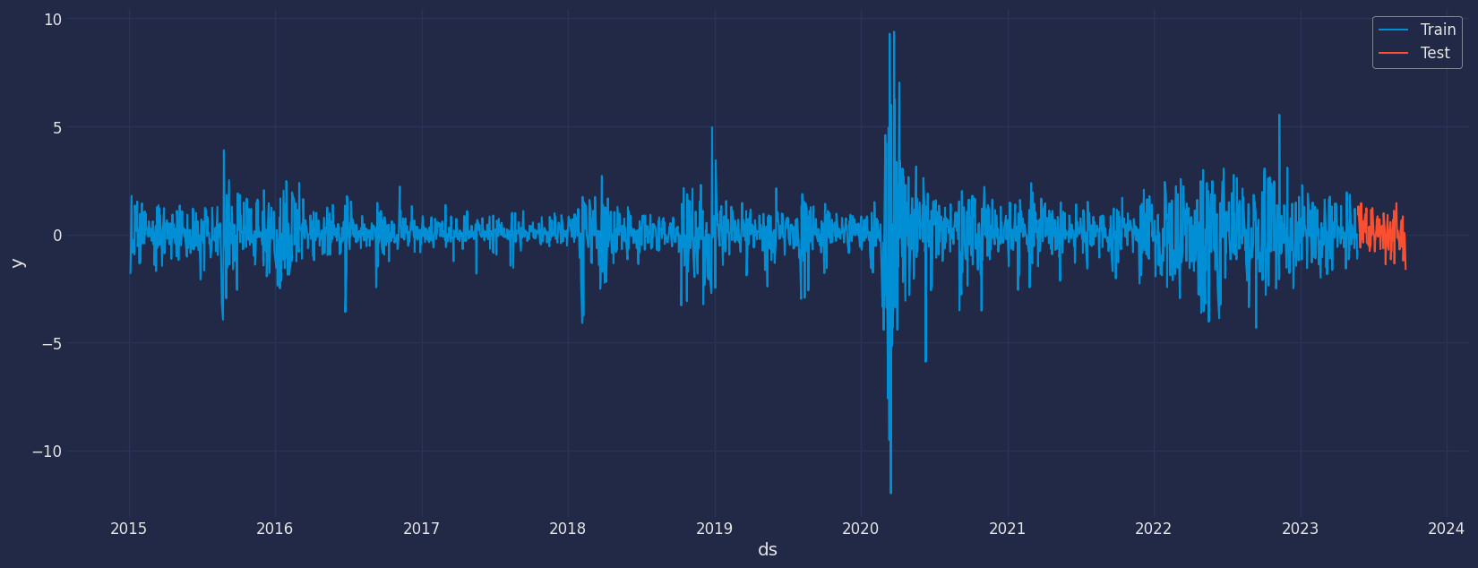
## Split the data into training and testing
Let’s divide our data into sets
1. Data to train our `ARCH` model
2. Data to test our model
For the test data we will use the last 30 day to test and evaluate the
performance of our model.
```python theme={null}
df=df[["ds","unique_id","return"]]
df.columns=["ds", "unique_id", "y"]
```
```python theme={null}
train = df[df.ds<='2023-05-24'] # Let's forecast the last 30 days
test = df[df.ds>'2023-05-24']
```
```python theme={null}
train.shape, test.shape
```
```text theme={null}
((2112, 3), (82, 3))
```
Now let’s plot the training data and the test data.
```python theme={null}
sns.lineplot(train,x="ds", y="y", label="Train")
sns.lineplot(test, x="ds", y="y", label="Test")
plt.show()
```
### Ljung-Box Test
Ljung-Box is a test for autocorrelation that we can use in tandem with
our ACF and PACF plots. The Ljung-Box test takes our data, optionally
either lag values to test, or the largest lag value to consider, and
whether to compute the Box-Pierce statistic. Ljung-Box and Box-Pierce
are two similar test statisitcs, Q , that are compared against a
chi-squared distribution to determine if the series is white noise. We
might use the Ljung-Box test on the residuals of our model to look for
autocorrelation, ideally our residuals would be white noise.
* Ho : The data are independently distributed, no autocorrelation.
* Ha : The data are not independently distributed; they exhibit serial
correlation.
The Ljung-Box with the Box-Pierce option will return, for each lag, the
Ljung-Box test statistic, Ljung-Box p-values, Box-Pierce test statistic,
and Box-Pierce p-values.
If $p<\alpha (0.05)$ we reject the null hypothesis.
```python theme={null}
from statsmodels.stats.diagnostic import acorr_ljungbox
ljung_res = acorr_ljungbox(df["return"], lags= 40, boxpierce=True)
ljung_res.head()
```
| | lb\_stat | lb\_pvalue | bp\_stat | bp\_pvalue |
| - | --------- | ------------ | --------- | ------------ |
| 1 | 49.222273 | 2.285409e-12 | 49.155183 | 2.364927e-12 |
| 2 | 62.991348 | 2.097020e-14 | 62.899234 | 2.195861e-14 |
| 3 | 63.944944 | 8.433622e-14 | 63.850663 | 8.834380e-14 |
| 4 | 74.343652 | 2.742989e-15 | 74.221024 | 2.911751e-15 |
| 5 | 80.234862 | 7.494100e-16 | 80.093498 | 8.022242e-16 |
## Split the data into training and testing
Let’s divide our data into sets
1. Data to train our `ARCH` model
2. Data to test our model
For the test data we will use the last 30 day to test and evaluate the
performance of our model.
```python theme={null}
df=df[["ds","unique_id","return"]]
df.columns=["ds", "unique_id", "y"]
```
```python theme={null}
train = df[df.ds<='2023-05-24'] # Let's forecast the last 30 days
test = df[df.ds>'2023-05-24']
```
```python theme={null}
train.shape, test.shape
```
```text theme={null}
((2112, 3), (82, 3))
```
Now let’s plot the training data and the test data.
```python theme={null}
sns.lineplot(train,x="ds", y="y", label="Train")
sns.lineplot(test, x="ds", y="y", label="Test")
plt.show()
```
 ## Implementation of ARCH with StatsForecast
To also know more about the parameters of the functions of the
`ARCH Model`, they are listed below. For more information, visit the
[documentation](../../src/core/models.html#arch)
```text theme={null}
p : int
Number of lagged versions of the series.
alias : str
Custom name of the model.
prediction_intervals : Optional[ConformalIntervals]
Information to compute conformal prediction intervals.
By default, the model will compute the native prediction
intervals.
```
### Load libraries
```python theme={null}
from statsforecast import StatsForecast
from statsforecast.models import ARCH
```
### Building Model
Import and instantiate the models. Setting the argument is sometimes
tricky. This article on [Seasonal
periods](https://robjhyndman.com/hyndsight/seasonal-periods/) by the
master, Rob Hyndmann, can be useful.season\_length.
```python theme={null}
season_length = 7 # Daily data
horizon = len(test) # number of predictions biasadj=True, include_drift=True,
models = [ARCH(p=2)]
```
We fit the models by instantiating a new StatsForecast object with the
following parameters:
models: a list of models. Select the models you want from models and
import them.
* `freq:` a string indicating the frequency of the data. (See [pandas’
available
frequencies](https://pandas.pydata.org/pandas-docs/stable/user_guide/timeseries.html#offset-aliases).)
* `n_jobs:` n\_jobs: int, number of jobs used in the parallel
processing, use -1 for all cores.
* `fallback_model:` a model to be used if a model fails.
Any settings are passed into the constructor. Then you call its fit
method and pass in the historical data frame.
```python theme={null}
sf = StatsForecast(models=models,
freq='C', # custom business day frequency
)
```
### Fit the Model
```python theme={null}
sf.fit(df=train)
```
```text theme={null}
StatsForecast(models=[ARCH(2)])
```
Let’s see the results of our ARCH model. We can observe it with the
following instruction:
```python theme={null}
result=sf.fitted_[0,0].model_
result
```
```text theme={null}
{'p': 2,
'q': 0,
'coeff': array([0.44321058, 0.34706751, 0.35172097]),
'message': 'Optimization terminated successfully',
'y_vals': array([-1.12220267, -0.73186003]),
'sigma2_vals': array([1.38768694, nan, 1.89278112, ..., 0.76423271, 0.45064684,
0.88037072]),
'fitted': array([ nan, nan, 2.23474807, ..., -1.48033228,
1.10018999, -0.98050166]),
'actual_residuals': array([ nan, nan, -1.07176381, ..., 1.49583575,
-2.22239266, 0.24864162])}
```
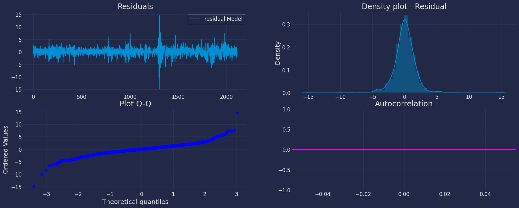
Let us now visualize the residuals of our models.
As we can see, the result obtained above has an output in a dictionary,
to extract each element from the dictionary we are going to use the
`.get()` function to extract the element and then we are going to save
it in a `pd.DataFrame()`.
```python theme={null}
residual=pd.DataFrame(result.get("actual_residuals"), columns=["residual Model"])
residual
```
| | residual Model |
| ---- | -------------- |
| 0 | NaN |
| 1 | NaN |
| 2 | -1.071764 |
| ... | ... |
| 2109 | 1.495836 |
| 2110 | -2.222393 |
| 2111 | 0.248642 |
```python theme={null}
import scipy.stats as stats
fig, axs = plt.subplots(nrows=2, ncols=2)
# plot[1,1]
residual.plot(ax=axs[0,0])
axs[0,0].set_title("Residuals");
# plot
sns.distplot(residual, ax=axs[0,1]);
axs[0,1].set_title("Density plot - Residual");
# plot
stats.probplot(residual["residual Model"], dist="norm", plot=axs[1,0])
axs[1,0].set_title('Plot Q-Q')
# plot
plot_acf(residual, lags=35, ax=axs[1,1],color="fuchsia")
axs[1,1].set_title("Autocorrelation");
plt.show();
```
## Implementation of ARCH with StatsForecast
To also know more about the parameters of the functions of the
`ARCH Model`, they are listed below. For more information, visit the
[documentation](../../src/core/models.html#arch)
```text theme={null}
p : int
Number of lagged versions of the series.
alias : str
Custom name of the model.
prediction_intervals : Optional[ConformalIntervals]
Information to compute conformal prediction intervals.
By default, the model will compute the native prediction
intervals.
```
### Load libraries
```python theme={null}
from statsforecast import StatsForecast
from statsforecast.models import ARCH
```
### Building Model
Import and instantiate the models. Setting the argument is sometimes
tricky. This article on [Seasonal
periods](https://robjhyndman.com/hyndsight/seasonal-periods/) by the
master, Rob Hyndmann, can be useful.season\_length.
```python theme={null}
season_length = 7 # Daily data
horizon = len(test) # number of predictions biasadj=True, include_drift=True,
models = [ARCH(p=2)]
```
We fit the models by instantiating a new StatsForecast object with the
following parameters:
models: a list of models. Select the models you want from models and
import them.
* `freq:` a string indicating the frequency of the data. (See [pandas’
available
frequencies](https://pandas.pydata.org/pandas-docs/stable/user_guide/timeseries.html#offset-aliases).)
* `n_jobs:` n\_jobs: int, number of jobs used in the parallel
processing, use -1 for all cores.
* `fallback_model:` a model to be used if a model fails.
Any settings are passed into the constructor. Then you call its fit
method and pass in the historical data frame.
```python theme={null}
sf = StatsForecast(models=models,
freq='C', # custom business day frequency
)
```
### Fit the Model
```python theme={null}
sf.fit(df=train)
```
```text theme={null}
StatsForecast(models=[ARCH(2)])
```
Let’s see the results of our ARCH model. We can observe it with the
following instruction:
```python theme={null}
result=sf.fitted_[0,0].model_
result
```
```text theme={null}
{'p': 2,
'q': 0,
'coeff': array([0.44321058, 0.34706751, 0.35172097]),
'message': 'Optimization terminated successfully',
'y_vals': array([-1.12220267, -0.73186003]),
'sigma2_vals': array([1.38768694, nan, 1.89278112, ..., 0.76423271, 0.45064684,
0.88037072]),
'fitted': array([ nan, nan, 2.23474807, ..., -1.48033228,
1.10018999, -0.98050166]),
'actual_residuals': array([ nan, nan, -1.07176381, ..., 1.49583575,
-2.22239266, 0.24864162])}
```
Let us now visualize the residuals of our models.
As we can see, the result obtained above has an output in a dictionary,
to extract each element from the dictionary we are going to use the
`.get()` function to extract the element and then we are going to save
it in a `pd.DataFrame()`.
```python theme={null}
residual=pd.DataFrame(result.get("actual_residuals"), columns=["residual Model"])
residual
```
| | residual Model |
| ---- | -------------- |
| 0 | NaN |
| 1 | NaN |
| 2 | -1.071764 |
| ... | ... |
| 2109 | 1.495836 |
| 2110 | -2.222393 |
| 2111 | 0.248642 |
```python theme={null}
import scipy.stats as stats
fig, axs = plt.subplots(nrows=2, ncols=2)
# plot[1,1]
residual.plot(ax=axs[0,0])
axs[0,0].set_title("Residuals");
# plot
sns.distplot(residual, ax=axs[0,1]);
axs[0,1].set_title("Density plot - Residual");
# plot
stats.probplot(residual["residual Model"], dist="norm", plot=axs[1,0])
axs[1,0].set_title('Plot Q-Q')
# plot
plot_acf(residual, lags=35, ax=axs[1,1],color="fuchsia")
axs[1,1].set_title("Autocorrelation");
plt.show();
```
 ### Forecast Method
If you want to gain speed in productive settings where you have multiple
series or models we recommend using the `StatsForecast.forecast` method
instead of `.fit` and `.predict`.
The main difference is that the `.forecast` doest not store the fitted
values and is highly scalable in distributed environments.
The forecast method takes two arguments: forecasts next `h` (horizon)
and `level`.
* `h (int):` represents the forecast h steps into the future. In this
case, 12 months ahead.
* `level (list of floats):` this optional parameter is used for
probabilistic forecasting. Set the level (or confidence percentile)
of your prediction interval. For example, `level=[90]` means that
the model expects the real value to be inside that interval 90% of
the times.
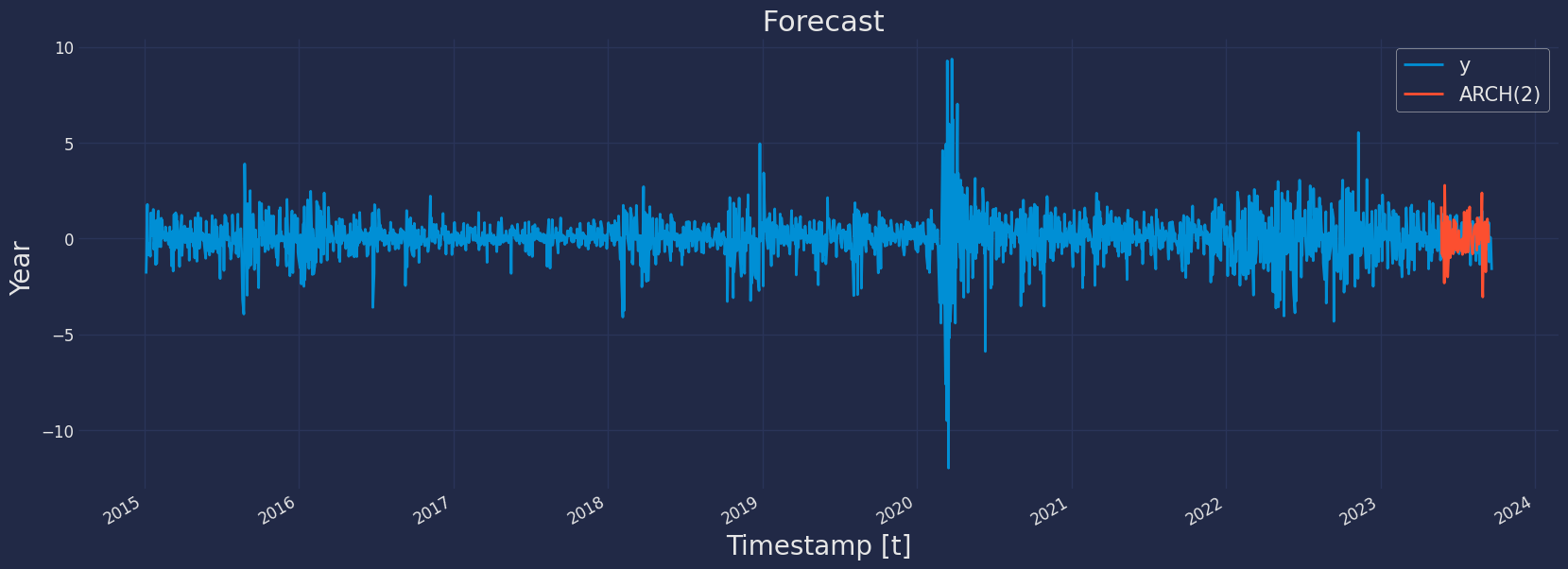
The forecast object here is a new data frame that includes a column with
the name of the model and the y hat values, as well as columns for the
uncertainty intervals. Depending on your computer, this step should take
around 1min.
```python theme={null}
Y_hat = sf.forecast(df=train, h=horizon, fitted=True)
Y_hat
```
| | unique\_id | ds | ARCH(2) |
| --- | ---------- | ------------------------- | --------- |
| 0 | 1 | 2023-05-25 00:00:00+00:00 | 1.681839 |
| 1 | 1 | 2023-05-26 00:00:00+00:00 | -0.777029 |
| 2 | 1 | 2023-05-29 00:00:00+00:00 | -0.677962 |
| ... | ... | ... | ... |
| 79 | 1 | 2023-09-13 00:00:00+00:00 | 0.695591 |
| 80 | 1 | 2023-09-14 00:00:00+00:00 | -0.176075 |
| 81 | 1 | 2023-09-15 00:00:00+00:00 | -0.158605 |
```python theme={null}
values=sf.forecast_fitted_values()
values.head()
```
| | unique\_id | ds | y | ARCH(2) |
| - | ---------- | ------------------------- | --------- | --------- |
| 0 | 1 | 2015-01-05 00:00:00+00:00 | -1.827811 | NaN |
| 1 | 1 | 2015-01-06 00:00:00+00:00 | -0.889347 | NaN |
| 2 | 1 | 2015-01-07 00:00:00+00:00 | 1.162984 | 2.234748 |
| 3 | 1 | 2015-01-08 00:00:00+00:00 | 1.788828 | -0.667577 |
| 4 | 1 | 2015-01-09 00:00:00+00:00 | -0.840381 | -0.752438 |
Adding 95% confidence interval with the forecast method
```python theme={null}
sf.forecast(df=train, h=horizon, level=[95])
```
| | unique\_id | ds | ARCH(2) | ARCH(2)-lo-95 | ARCH(2)-hi-95 |
| --- | ---------- | ------------------------- | --------- | ------------- | ------------- |
| 0 | 1 | 2023-05-25 00:00:00+00:00 | 1.681839 | -0.419326 | 3.783003 |
| 1 | 1 | 2023-05-26 00:00:00+00:00 | -0.777029 | -3.939054 | 2.384996 |
| 2 | 1 | 2023-05-29 00:00:00+00:00 | -0.677962 | -3.907262 | 2.551338 |
| ... | ... | ... | ... | ... | ... |
| 79 | 1 | 2023-09-13 00:00:00+00:00 | 0.695591 | -0.937585 | 2.328766 |
| 80 | 1 | 2023-09-14 00:00:00+00:00 | -0.176075 | -1.405359 | 1.053210 |
| 81 | 1 | 2023-09-15 00:00:00+00:00 | -0.158605 | -1.381915 | 1.064705 |
```python theme={null}
# Merge the forecasts with the true values
Y_hat1 = test.merge(Y_hat, how='left', on=['unique_id', 'ds'])
Y_hat1
```
| | ds | unique\_id | y | ARCH(2) |
| --- | ------------------------- | ---------- | --------- | --------- |
| 0 | 2023-05-25 00:00:00+00:00 | 1 | 0.875758 | 1.681839 |
| 1 | 2023-05-26 00:00:00+00:00 | 1 | 1.304909 | -0.777029 |
| 2 | 2023-05-30 00:00:00+00:00 | 1 | 0.001660 | -0.968703 |
| ... | ... | ... | ... | ... |
| 79 | 2023-09-19 00:00:00+00:00 | 1 | -0.215101 | NaN |
| 80 | 2023-09-20 00:00:00+00:00 | 1 | -0.939479 | NaN |
| 81 | 2023-09-21 00:00:00+00:00 | 1 | -1.640093 | NaN |
```python theme={null}
# Merge the forecasts with the true values
fig, ax = plt.subplots(1, 1)
plot_df = pd.concat([train, Y_hat1]).set_index('ds')
plot_df[['y', "ARCH(2)"]].plot(ax=ax, linewidth=2)
ax.set_title(' Forecast', fontsize=22)
ax.set_ylabel('Year ', fontsize=20)
ax.set_xlabel('Timestamp [t]', fontsize=20)
ax.legend(prop={'size': 15})
ax.grid(True)
plt.show()
```
### Forecast Method
If you want to gain speed in productive settings where you have multiple
series or models we recommend using the `StatsForecast.forecast` method
instead of `.fit` and `.predict`.
The main difference is that the `.forecast` doest not store the fitted
values and is highly scalable in distributed environments.
The forecast method takes two arguments: forecasts next `h` (horizon)
and `level`.
* `h (int):` represents the forecast h steps into the future. In this
case, 12 months ahead.
* `level (list of floats):` this optional parameter is used for
probabilistic forecasting. Set the level (or confidence percentile)
of your prediction interval. For example, `level=[90]` means that
the model expects the real value to be inside that interval 90% of
the times.
The forecast object here is a new data frame that includes a column with
the name of the model and the y hat values, as well as columns for the
uncertainty intervals. Depending on your computer, this step should take
around 1min.
```python theme={null}
Y_hat = sf.forecast(df=train, h=horizon, fitted=True)
Y_hat
```
| | unique\_id | ds | ARCH(2) |
| --- | ---------- | ------------------------- | --------- |
| 0 | 1 | 2023-05-25 00:00:00+00:00 | 1.681839 |
| 1 | 1 | 2023-05-26 00:00:00+00:00 | -0.777029 |
| 2 | 1 | 2023-05-29 00:00:00+00:00 | -0.677962 |
| ... | ... | ... | ... |
| 79 | 1 | 2023-09-13 00:00:00+00:00 | 0.695591 |
| 80 | 1 | 2023-09-14 00:00:00+00:00 | -0.176075 |
| 81 | 1 | 2023-09-15 00:00:00+00:00 | -0.158605 |
```python theme={null}
values=sf.forecast_fitted_values()
values.head()
```
| | unique\_id | ds | y | ARCH(2) |
| - | ---------- | ------------------------- | --------- | --------- |
| 0 | 1 | 2015-01-05 00:00:00+00:00 | -1.827811 | NaN |
| 1 | 1 | 2015-01-06 00:00:00+00:00 | -0.889347 | NaN |
| 2 | 1 | 2015-01-07 00:00:00+00:00 | 1.162984 | 2.234748 |
| 3 | 1 | 2015-01-08 00:00:00+00:00 | 1.788828 | -0.667577 |
| 4 | 1 | 2015-01-09 00:00:00+00:00 | -0.840381 | -0.752438 |
Adding 95% confidence interval with the forecast method
```python theme={null}
sf.forecast(df=train, h=horizon, level=[95])
```
| | unique\_id | ds | ARCH(2) | ARCH(2)-lo-95 | ARCH(2)-hi-95 |
| --- | ---------- | ------------------------- | --------- | ------------- | ------------- |
| 0 | 1 | 2023-05-25 00:00:00+00:00 | 1.681839 | -0.419326 | 3.783003 |
| 1 | 1 | 2023-05-26 00:00:00+00:00 | -0.777029 | -3.939054 | 2.384996 |
| 2 | 1 | 2023-05-29 00:00:00+00:00 | -0.677962 | -3.907262 | 2.551338 |
| ... | ... | ... | ... | ... | ... |
| 79 | 1 | 2023-09-13 00:00:00+00:00 | 0.695591 | -0.937585 | 2.328766 |
| 80 | 1 | 2023-09-14 00:00:00+00:00 | -0.176075 | -1.405359 | 1.053210 |
| 81 | 1 | 2023-09-15 00:00:00+00:00 | -0.158605 | -1.381915 | 1.064705 |
```python theme={null}
# Merge the forecasts with the true values
Y_hat1 = test.merge(Y_hat, how='left', on=['unique_id', 'ds'])
Y_hat1
```
| | ds | unique\_id | y | ARCH(2) |
| --- | ------------------------- | ---------- | --------- | --------- |
| 0 | 2023-05-25 00:00:00+00:00 | 1 | 0.875758 | 1.681839 |
| 1 | 2023-05-26 00:00:00+00:00 | 1 | 1.304909 | -0.777029 |
| 2 | 2023-05-30 00:00:00+00:00 | 1 | 0.001660 | -0.968703 |
| ... | ... | ... | ... | ... |
| 79 | 2023-09-19 00:00:00+00:00 | 1 | -0.215101 | NaN |
| 80 | 2023-09-20 00:00:00+00:00 | 1 | -0.939479 | NaN |
| 81 | 2023-09-21 00:00:00+00:00 | 1 | -1.640093 | NaN |
```python theme={null}
# Merge the forecasts with the true values
fig, ax = plt.subplots(1, 1)
plot_df = pd.concat([train, Y_hat1]).set_index('ds')
plot_df[['y', "ARCH(2)"]].plot(ax=ax, linewidth=2)
ax.set_title(' Forecast', fontsize=22)
ax.set_ylabel('Year ', fontsize=20)
ax.set_xlabel('Timestamp [t]', fontsize=20)
ax.legend(prop={'size': 15})
ax.grid(True)
plt.show()
```
 ### Predict method with confidence interval
To generate forecasts use the predict method.
The predict method takes two arguments: forecasts the next `h` (for
horizon) and `level`.
* `h (int):` represents the forecast h steps into the future. In this
case, 12 months ahead.
* `level (list of floats):` this optional parameter is used for
probabilistic forecasting. Set the level (or confidence percentile)
of your prediction interval. For example, `level=[95]` means that
the model expects the real value to be inside that interval 95% of
the times.
The forecast object here is a new data frame that includes a column with
the name of the model and the y hat values, as well as columns for the
uncertainty intervals.
This step should take less than 1 second.
```python theme={null}
sf.predict(h=horizon)
```
| | unique\_id | ds | ARCH(2) |
| --- | ---------- | ------------------------- | --------- |
| 0 | 1 | 2023-05-25 00:00:00+00:00 | 1.681839 |
| 1 | 1 | 2023-05-26 00:00:00+00:00 | -0.777029 |
| 2 | 1 | 2023-05-29 00:00:00+00:00 | -0.677962 |
| ... | ... | ... | ... |
| 79 | 1 | 2023-09-13 00:00:00+00:00 | 0.695591 |
| 80 | 1 | 2023-09-14 00:00:00+00:00 | -0.176075 |
| 81 | 1 | 2023-09-15 00:00:00+00:00 | -0.158605 |
```python theme={null}
forecast_df = sf.predict(h=horizon, level=[80,95])
forecast_df
```
| | unique\_id | ds | ARCH(2) | ARCH(2)-lo-95 | ARCH(2)-lo-80 | ARCH(2)-hi-80 | ARCH(2)-hi-95 |
| --- | ---------- | ------------------------- | --------- | ------------- | ------------- | ------------- | ------------- |
| 0 | 1 | 2023-05-25 00:00:00+00:00 | 1.681839 | -0.419326 | 0.307961 | 3.055716 | 3.783003 |
| 1 | 1 | 2023-05-26 00:00:00+00:00 | -0.777029 | -3.939054 | -2.844566 | 1.290508 | 2.384996 |
| 2 | 1 | 2023-05-29 00:00:00+00:00 | -0.677962 | -3.907262 | -2.789488 | 1.433564 | 2.551338 |
| ... | ... | ... | ... | ... | ... | ... | ... |
| 79 | 1 | 2023-09-13 00:00:00+00:00 | 0.695591 | -0.937585 | -0.372285 | 1.763467 | 2.328766 |
| 80 | 1 | 2023-09-14 00:00:00+00:00 | -0.176075 | -1.405359 | -0.979860 | 0.627711 | 1.053210 |
| 81 | 1 | 2023-09-15 00:00:00+00:00 | -0.158605 | -1.381915 | -0.958485 | 0.641274 | 1.064705 |
We can join the forecast result with the historical data using the
pandas function `pd.concat()`, and then be able to use this result for
graphing.
```python theme={null}
df_plot=pd.concat([df, forecast_df]).set_index('ds').tail(220)
df_plot
```
| | unique\_id | y | ARCH(2) | ARCH(2)-lo-95 | ARCH(2)-lo-80 | ARCH(2)-hi-80 | ARCH(2)-hi-95 |
| ------------------------- | ---------- | --------- | --------- | ------------- | ------------- | ------------- | ------------- |
| ds | | | | | | | |
| 2023-03-07 00:00:00+00:00 | 1 | -1.532692 | NaN | NaN | NaN | NaN | NaN |
| 2023-03-08 00:00:00+00:00 | 1 | 0.141479 | NaN | NaN | NaN | NaN | NaN |
| 2023-03-09 00:00:00+00:00 | 1 | -1.845936 | NaN | NaN | NaN | NaN | NaN |
| ... | ... | ... | ... | ... | ... | ... | ... |
| 2023-09-13 00:00:00+00:00 | 1 | NaN | 0.695591 | -0.937585 | -0.372285 | 1.763467 | 2.328766 |
| 2023-09-14 00:00:00+00:00 | 1 | NaN | -0.176075 | -1.405359 | -0.979860 | 0.627711 | 1.053210 |
| 2023-09-15 00:00:00+00:00 | 1 | NaN | -0.158605 | -1.381915 | -0.958485 | 0.641274 | 1.064705 |
```python theme={null}
sf.plot(train, test.merge(forecast_df), level=[80, 95], max_insample_length=120)
```
### Predict method with confidence interval
To generate forecasts use the predict method.
The predict method takes two arguments: forecasts the next `h` (for
horizon) and `level`.
* `h (int):` represents the forecast h steps into the future. In this
case, 12 months ahead.
* `level (list of floats):` this optional parameter is used for
probabilistic forecasting. Set the level (or confidence percentile)
of your prediction interval. For example, `level=[95]` means that
the model expects the real value to be inside that interval 95% of
the times.
The forecast object here is a new data frame that includes a column with
the name of the model and the y hat values, as well as columns for the
uncertainty intervals.
This step should take less than 1 second.
```python theme={null}
sf.predict(h=horizon)
```
| | unique\_id | ds | ARCH(2) |
| --- | ---------- | ------------------------- | --------- |
| 0 | 1 | 2023-05-25 00:00:00+00:00 | 1.681839 |
| 1 | 1 | 2023-05-26 00:00:00+00:00 | -0.777029 |
| 2 | 1 | 2023-05-29 00:00:00+00:00 | -0.677962 |
| ... | ... | ... | ... |
| 79 | 1 | 2023-09-13 00:00:00+00:00 | 0.695591 |
| 80 | 1 | 2023-09-14 00:00:00+00:00 | -0.176075 |
| 81 | 1 | 2023-09-15 00:00:00+00:00 | -0.158605 |
```python theme={null}
forecast_df = sf.predict(h=horizon, level=[80,95])
forecast_df
```
| | unique\_id | ds | ARCH(2) | ARCH(2)-lo-95 | ARCH(2)-lo-80 | ARCH(2)-hi-80 | ARCH(2)-hi-95 |
| --- | ---------- | ------------------------- | --------- | ------------- | ------------- | ------------- | ------------- |
| 0 | 1 | 2023-05-25 00:00:00+00:00 | 1.681839 | -0.419326 | 0.307961 | 3.055716 | 3.783003 |
| 1 | 1 | 2023-05-26 00:00:00+00:00 | -0.777029 | -3.939054 | -2.844566 | 1.290508 | 2.384996 |
| 2 | 1 | 2023-05-29 00:00:00+00:00 | -0.677962 | -3.907262 | -2.789488 | 1.433564 | 2.551338 |
| ... | ... | ... | ... | ... | ... | ... | ... |
| 79 | 1 | 2023-09-13 00:00:00+00:00 | 0.695591 | -0.937585 | -0.372285 | 1.763467 | 2.328766 |
| 80 | 1 | 2023-09-14 00:00:00+00:00 | -0.176075 | -1.405359 | -0.979860 | 0.627711 | 1.053210 |
| 81 | 1 | 2023-09-15 00:00:00+00:00 | -0.158605 | -1.381915 | -0.958485 | 0.641274 | 1.064705 |
We can join the forecast result with the historical data using the
pandas function `pd.concat()`, and then be able to use this result for
graphing.
```python theme={null}
df_plot=pd.concat([df, forecast_df]).set_index('ds').tail(220)
df_plot
```
| | unique\_id | y | ARCH(2) | ARCH(2)-lo-95 | ARCH(2)-lo-80 | ARCH(2)-hi-80 | ARCH(2)-hi-95 |
| ------------------------- | ---------- | --------- | --------- | ------------- | ------------- | ------------- | ------------- |
| ds | | | | | | | |
| 2023-03-07 00:00:00+00:00 | 1 | -1.532692 | NaN | NaN | NaN | NaN | NaN |
| 2023-03-08 00:00:00+00:00 | 1 | 0.141479 | NaN | NaN | NaN | NaN | NaN |
| 2023-03-09 00:00:00+00:00 | 1 | -1.845936 | NaN | NaN | NaN | NaN | NaN |
| ... | ... | ... | ... | ... | ... | ... | ... |
| 2023-09-13 00:00:00+00:00 | 1 | NaN | 0.695591 | -0.937585 | -0.372285 | 1.763467 | 2.328766 |
| 2023-09-14 00:00:00+00:00 | 1 | NaN | -0.176075 | -1.405359 | -0.979860 | 0.627711 | 1.053210 |
| 2023-09-15 00:00:00+00:00 | 1 | NaN | -0.158605 | -1.381915 | -0.958485 | 0.641274 | 1.064705 |
```python theme={null}
sf.plot(train, test.merge(forecast_df), level=[80, 95], max_insample_length=120)
```
 Let’s plot the same graph using the plot function that comes in
`Statsforecast`, as shown below.
## Cross-validation
In previous steps, we’ve taken our historical data to predict the
future. However, to asses its accuracy we would also like to know how
the model would have performed in the past. To assess the accuracy and
robustness of your models on your data perform Cross-Validation.
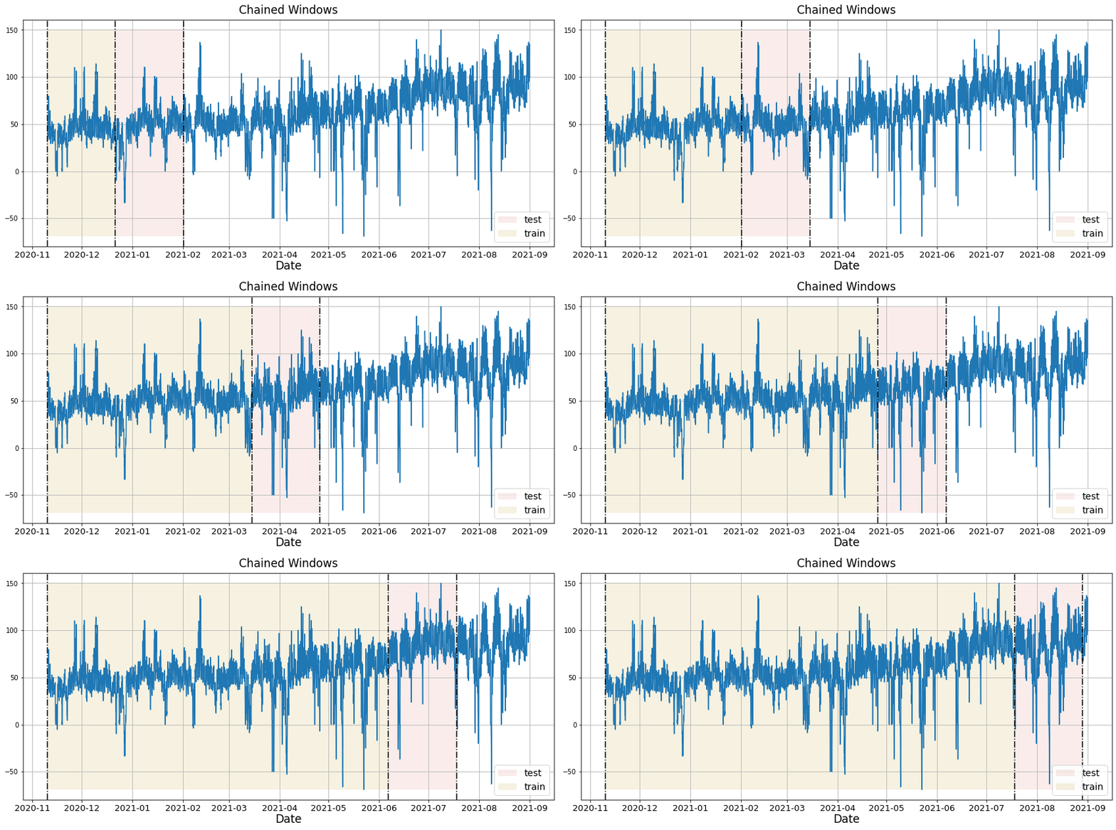
With time series data, Cross Validation is done by defining a sliding
window across the historical data and predicting the period following
it. This form of cross-validation allows us to arrive at a better
estimation of our model’s predictive abilities across a wider range of
temporal instances while also keeping the data in the training set
contiguous as is required by our models.
The following graph depicts such a Cross Validation Strategy:
### Perform time series cross-validation
Cross-validation of time series models is considered a best practice but
most implementations are very slow. The statsforecast library implements
cross-validation as a distributed operation, making the process less
time-consuming to perform. If you have big datasets you can also perform
Cross Validation in a distributed cluster using Ray, Dask or Spark.
In this case, we want to evaluate the performance of each model for the
last 5 months `(n_windows=5)`, forecasting every second months
`(step_size=12)`. Depending on your computer, this step should take
around 1 min.
The cross\_validation method from the StatsForecast class takes the
following arguments.
* `df:` training data frame
* `h (int):` represents h steps into the future that are being
forecasted. In this case, 12 months ahead.
* `step_size (int):` step size between each window. In other words:
how often do you want to run the forecasting processes.
* `n_windows(int):` number of windows used for cross validation. In
other words: what number of forecasting processes in the past do you
want to evaluate.
```python theme={null}
crossvalidation_df = sf.cross_validation(df=train,
h=horizon,
step_size=6,
n_windows=5)
```
The crossvaldation\_df object is a new data frame that includes the
following columns:
* `unique_id:` series identifier
* `ds:` datestamp or temporal index
* `cutoff:` the last datestamp or temporal index for the n\_windows.
* `y:` true value
* `"model":` columns with the model’s name and fitted value.
```python theme={null}
crossvalidation_df
```
| | unique\_id | ds | cutoff | y | ARCH(2) |
| --- | ---------- | ------------------------- | ------------------------- | --------- | --------- |
| 0 | 1 | 2022-12-21 00:00:00+00:00 | 2022-12-20 00:00:00+00:00 | 1.486799 | 1.382105 |
| 1 | 1 | 2022-12-22 00:00:00+00:00 | 2022-12-20 00:00:00+00:00 | -1.445170 | -0.651618 |
| 2 | 1 | 2022-12-23 00:00:00+00:00 | 2022-12-20 00:00:00+00:00 | 0.586810 | -0.595213 |
| ... | ... | ... | ... | ... | ... |
| 407 | 1 | 2023-05-22 00:00:00+00:00 | 2023-01-26 00:00:00+00:00 | 0.015503 | 0.693070 |
| 408 | 1 | 2023-05-23 00:00:00+00:00 | 2023-01-26 00:00:00+00:00 | -1.122203 | -0.176181 |
| 409 | 1 | 2023-05-24 00:00:00+00:00 | 2023-01-26 00:00:00+00:00 | -0.731860 | -0.157522 |
## Model Evaluation
Now we are going to evaluate our model with the results of the
predictions, we will use different types of metrics MAE, MAPE, MASE,
RMSE, SMAPE to evaluate the accuracy.
```python theme={null}
from functools import partial
from utilsforecast.evaluation import evaluate
from utilsforecast.losses import mae, mape, mase, rmse, smape
```
```python theme={null}
evaluate(
test.merge(Y_hat),
train_df=train,
metrics=[mae, mape, partial(mase, seasonality=5), rmse, smape],
agg_fn='mean',
)
```
| | metric | ARCH(2) |
| - | ------ | --------- |
| 0 | mae | 0.949721 |
| 1 | mape | 11.789856 |
| 2 | mase | 0.875298 |
| 3 | rmse | 1.164914 |
| 4 | smape | 0.725702 |
## References
1. [Changquan Huang • Alla Petukhina. Springer series (2022). Applied
Time Series Analysis and Forecasting with
Python.](https://link.springer.com/book/10.1007/978-3-031-13584-2)
2. [Engle, R. F. (1982). Autoregressive conditional heteroscedasticity
with estimates of the variance of United Kingdom inflation.
Econometrica: Journal of the econometric society,
987-1007.](http://www.econ.uiuc.edu/~econ508/Papers/engle82.pdf).
3. [James D. Hamilton. Time Series Analysis Princeton University Press,
Princeton, New Jersey, 1st Edition,
1994.](https://press.princeton.edu/books/hardcover/9780691042893/time-series-analysis)
4. [Nixtla ARCH API](../../src/core/models.html#arch)
5. [Pandas available
frequencies](https://pandas.pydata.org/pandas-docs/stable/user_guide/timeseries.html#offset-aliases).
6. [Rob J. Hyndman and George Athanasopoulos (2018). “Forecasting
Principles and Practice (3rd
ed)”](https://otexts.com/fpp3/tscv.html).
7. [Seasonal periods- Rob J
Hyndman](https://robjhyndman.com/hyndsight/seasonal-periods/).
Let’s plot the same graph using the plot function that comes in
`Statsforecast`, as shown below.
## Cross-validation
In previous steps, we’ve taken our historical data to predict the
future. However, to asses its accuracy we would also like to know how
the model would have performed in the past. To assess the accuracy and
robustness of your models on your data perform Cross-Validation.
With time series data, Cross Validation is done by defining a sliding
window across the historical data and predicting the period following
it. This form of cross-validation allows us to arrive at a better
estimation of our model’s predictive abilities across a wider range of
temporal instances while also keeping the data in the training set
contiguous as is required by our models.
The following graph depicts such a Cross Validation Strategy:

### Perform time series cross-validation
Cross-validation of time series models is considered a best practice but
most implementations are very slow. The statsforecast library implements
cross-validation as a distributed operation, making the process less
time-consuming to perform. If you have big datasets you can also perform
Cross Validation in a distributed cluster using Ray, Dask or Spark.
In this case, we want to evaluate the performance of each model for the
last 5 months `(n_windows=5)`, forecasting every second months
`(step_size=12)`. Depending on your computer, this step should take
around 1 min.
The cross\_validation method from the StatsForecast class takes the
following arguments.
* `df:` training data frame
* `h (int):` represents h steps into the future that are being
forecasted. In this case, 12 months ahead.
* `step_size (int):` step size between each window. In other words:
how often do you want to run the forecasting processes.
* `n_windows(int):` number of windows used for cross validation. In
other words: what number of forecasting processes in the past do you
want to evaluate.
```python theme={null}
crossvalidation_df = sf.cross_validation(df=train,
h=horizon,
step_size=6,
n_windows=5)
```
The crossvaldation\_df object is a new data frame that includes the
following columns:
* `unique_id:` series identifier
* `ds:` datestamp or temporal index
* `cutoff:` the last datestamp or temporal index for the n\_windows.
* `y:` true value
* `"model":` columns with the model’s name and fitted value.
```python theme={null}
crossvalidation_df
```
| | unique\_id | ds | cutoff | y | ARCH(2) |
| --- | ---------- | ------------------------- | ------------------------- | --------- | --------- |
| 0 | 1 | 2022-12-21 00:00:00+00:00 | 2022-12-20 00:00:00+00:00 | 1.486799 | 1.382105 |
| 1 | 1 | 2022-12-22 00:00:00+00:00 | 2022-12-20 00:00:00+00:00 | -1.445170 | -0.651618 |
| 2 | 1 | 2022-12-23 00:00:00+00:00 | 2022-12-20 00:00:00+00:00 | 0.586810 | -0.595213 |
| ... | ... | ... | ... | ... | ... |
| 407 | 1 | 2023-05-22 00:00:00+00:00 | 2023-01-26 00:00:00+00:00 | 0.015503 | 0.693070 |
| 408 | 1 | 2023-05-23 00:00:00+00:00 | 2023-01-26 00:00:00+00:00 | -1.122203 | -0.176181 |
| 409 | 1 | 2023-05-24 00:00:00+00:00 | 2023-01-26 00:00:00+00:00 | -0.731860 | -0.157522 |
## Model Evaluation
Now we are going to evaluate our model with the results of the
predictions, we will use different types of metrics MAE, MAPE, MASE,
RMSE, SMAPE to evaluate the accuracy.
```python theme={null}
from functools import partial
from utilsforecast.evaluation import evaluate
from utilsforecast.losses import mae, mape, mase, rmse, smape
```
```python theme={null}
evaluate(
test.merge(Y_hat),
train_df=train,
metrics=[mae, mape, partial(mase, seasonality=5), rmse, smape],
agg_fn='mean',
)
```
| | metric | ARCH(2) |
| - | ------ | --------- |
| 0 | mae | 0.949721 |
| 1 | mape | 11.789856 |
| 2 | mase | 0.875298 |
| 3 | rmse | 1.164914 |
| 4 | smape | 0.725702 |
## References
1. [Changquan Huang • Alla Petukhina. Springer series (2022). Applied
Time Series Analysis and Forecasting with
Python.](https://link.springer.com/book/10.1007/978-3-031-13584-2)
2. [Engle, R. F. (1982). Autoregressive conditional heteroscedasticity
with estimates of the variance of United Kingdom inflation.
Econometrica: Journal of the econometric society,
987-1007.](http://www.econ.uiuc.edu/~econ508/Papers/engle82.pdf).
3. [James D. Hamilton. Time Series Analysis Princeton University Press,
Princeton, New Jersey, 1st Edition,
1994.](https://press.princeton.edu/books/hardcover/9780691042893/time-series-analysis)
4. [Nixtla ARCH API](../../src/core/models.html#arch)
5. [Pandas available
frequencies](https://pandas.pydata.org/pandas-docs/stable/user_guide/timeseries.html#offset-aliases).
6. [Rob J. Hyndman and George Athanasopoulos (2018). “Forecasting
Principles and Practice (3rd
ed)”](https://otexts.com/fpp3/tscv.html).
7. [Seasonal periods- Rob J
Hyndman](https://robjhyndman.com/hyndsight/seasonal-periods/).