> ## Documentation Index
> Fetch the complete documentation index at: https://nixtlaverse.nixtla.io/llms.txt
> Use this file to discover all available pages before exploring further.
# End to End Walkthrough with Polars
> Model training, evaluation and selection for multiple time series
## Introducing Polars: A High-Performance DataFrame Library
This document aims to highlight the recent integration of Polars, a
robust and high-speed DataFrame library developed in Rust, into the
functionality of StatsForecast. Polars, with its nimble and potent
capabilities, has rapidly established a strong reputation within the
Data Science community, further solidifying its position as a reliable
tool for managing and manipulating substantial data sets.
Available in languages including Rust, Python, Node.js, and R, Polars
demonstrates a remarkable ability to handle sizable data sets with
efficiency and speed that surpasses many other DataFrame libraries, such
as Pandas. Polars’ open-source nature invites ongoing enhancements and
contributions, augmenting its appeal within the data science arena.
The most significant features of Polars that contribute to its rapid
adoption are:
1. **Performance Efficiency**: Constructed using Rust, Polars exhibits
an exemplary ability to manage substantial datasets with remarkable
speed and minimal memory usage.
2. **Lazy Evaluation**: Polars operates on the principle of ‘lazy
evaluation’, creating an optimized logical plan of operations for
efficient execution, a feature that mirrors the functionality of
Apache Spark.
3. **Parallel Execution**: Demonstrating the capability to exploit
multi-core CPUs, Polars facilitates parallel execution of
operations, substantially accelerating data processing tasks.
> **Prerequisites**
>
> This Guide assumes basic familiarity with StatsForecast. For a minimal
> example visit the [Quick Start](./getting_started_short.html)
Follow this article for a step-by-step guide on building a
production-ready forecasting pipeline for multiple time series.
During this guide you will gain familiarity with the core
`StatsForecast`class and some relevant methods like
`StatsForecast.plot`, `StatsForecast.forecast` and
`StatsForecast.cross_validation.`
We will use a classical benchmarking dataset from the M4 competition.
The dataset includes time series from different domains like finance,
economy and sales. In this example, we will use a subset of the Hourly
dataset.
We will model each time series individually. Forecasting at this level
is also known as local forecasting. Therefore, you will train a series
of models for every unique series and then select the best one.
StatsForecast focuses on speed, simplicity, and scalability, which makes
it ideal for this task.
**Outline:**
1. Install packages.
2. Read the data.
3. Explore the data.
4. Train many models for every unique combination of time series.
5. Evaluate the model’s performance using cross-validation.
6. Select the best model for every unique time series.
> **Not Covered in this guide**
>
> * Forecasting at scale using clusters on the cloud.
> * [Forecast the M5 Dataset in
> 5min](../experiments/ets_ray_m5.html) using Ray clusters.
> * [Forecast the M5 Dataset in
> 5min](../experiments/prophet_spark_m5.html) using Spark
> clusters.
> * Learn how to predict [1M series in less than
> 30min](https://www.anyscale.com/blog/how-nixtla-uses-ray-to-accurately-predict-more-than-a-million-time-series).
> * Training models on Multiple Seasonalities.
> * Learn to use multiple seasonality in this [Electricity Load
> forecasting](../tutorials/electricityloadforecasting.html)
> tutorial.
> * Using external regressors or exogenous variables
> * Follow this tutorial to [include exogenous
> variables](../how-to-guides/exogenous.html) like weather or
> holidays or static variables like category or family.
> * Comparing StatsForecast with other popular libraries.
> * You can reproduce our benchmarks
> [here](https://github.com/Nixtla/statsforecast/tree/main/experiments).
## Install libraries
We assume you have StatsForecast already installed. Check this guide for
instructions on [how to install StatsForecast](./installation.html).
## Read the data
We will use polars to read the M4 Hourly data set stored in a parquet
file for efficiency. You can use ordinary polars operations to read your
data in other formats likes `.csv`.
The input to StatsForecast is always a data frame in [long
format](https://www.theanalysisfactor.com/wide-and-long-data/) with
three columns: `unique_id`, `ds` and `y`:
* The `unique_id` (string, int or category) represents an identifier
for the series.
* The `ds` (datestamp or int) column should be either an integer
indexing time or a datestamp ideally like YYYY-MM-DD for a date or
YYYY-MM-DD HH:MM:SS for a timestamp.
* The `y` (numeric) represents the measurement we wish to forecast.
This data set already satisfies the requirement.
Depending on your internet connection, this step should take around 10
seconds.
```python theme={null}
import polars as pl
```
```python theme={null}
Y_df = pl.read_parquet('https://datasets-nixtla.s3.amazonaws.com/m4-hourly.parquet')
Y_df.head()
```
| unique\_id | ds | y |
| ---------- | --- | ----- |
| str | i64 | f64 |
| "H1" | 1 | 605.0 |
| "H1" | 2 | 586.0 |
| "H1" | 3 | 586.0 |
| "H1" | 4 | 559.0 |
| "H1" | 5 | 511.0 |
This dataset contains 414 unique series with 900 observations on
average. For this example and reproducibility’s sake, we will select
only 10 unique IDs and keep only the last week. Depending on your
processing infrastructure feel free to select more or less series.
> **Note**
>
> Processing time is dependent on the available computing resources.
> Running this example with the complete dataset takes around 10 minutes
> in a c5d.24xlarge (96 cores) instance from AWS.
```python theme={null}
uids = Y_df['unique_id'].unique(maintain_order=True)[:10] # Select 10 ids to make the example faster
Y_df = Y_df.filter(pl.col('unique_id').is_in(uids))
Y_df = Y_df.group_by('unique_id').tail(7 * 24) #Select last 7 days of data to make example faster
```
```text theme={null}
/var/folders/cc/cylsfhls0hb_9wg0wh8tvpyh0000gn/T/ipykernel_32103/3020671980.py:2: DeprecationWarning: `is_in` with a collection of the same datatype is ambiguous and deprecated.
Please use `implode` to return to previous behavior.
See https://github.com/pola-rs/polars/issues/22149 for more information.
Y_df = Y_df.filter(pl.col('unique_id').is_in(uids))
```
## Explore Data with the plot method
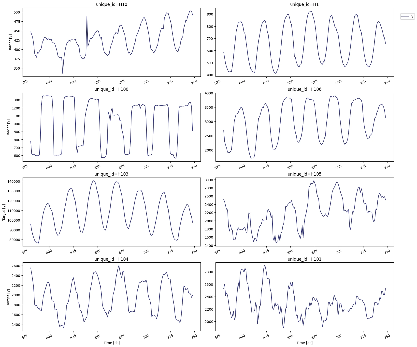
Plot some series using the `plot` method from the `StatsForecast` class.
This method prints 8 random series from the dataset and is useful for
basic EDA.
> **Note**
>
> The `StatsForecast.plot` method uses matplotlib as a default engine.
> You can change to plotly by setting `engine="plotly"`.
```python theme={null}
from statsforecast import StatsForecast
```
```text theme={null}
/Users/nasaul/nixtla/statsforecast/.venv/lib/python3.9/site-packages/tqdm/auto.py:21: TqdmWarning: IProgress not found. Please update jupyter and ipywidgets. See https://ipywidgets.readthedocs.io/en/stable/user_install.html
from .autonotebook import tqdm as notebook_tqdm
```
```python theme={null}
StatsForecast.plot(Y_df)
```
 ## Train multiple models for many series
StatsForecast can train many models on many time series efficiently.
Start by importing and instantiating the desired models. StatsForecast
offers a wide variety of models grouped in the following categories:
* **Auto Forecast:** Automatic forecasting tools search for the best
parameters and select the best possible model for a series of time
series. These tools are useful for large collections of univariate
time series. Includes automatic versions of: Arima, ETS, Theta, CES.
* **Exponential Smoothing:** Uses a weighted average of all past
observations where the weights decrease exponentially into the past.
Suitable for data with no clear trend or seasonality. Examples: SES,
Holt’s Winters, SSO.
* **Benchmark models:** classical models for establishing baselines.
Examples: Mean, Naive, Random Walk
* **Intermittent or Sparse models:** suited for series with very few
non-zero observations. Examples: CROSTON, ADIDA, IMAPA
* **Multiple Seasonalities:** suited for signals with more than one
clear seasonality. Useful for low-frequency data like electricity
and logs. Examples: MSTL.
* **Theta Models:** fit two theta lines to a deseasonalized time
series, using different techniques to obtain and combine the two
theta lines to produce the final forecasts. Examples: Theta,
DynamicTheta
Here you can check the complete list of
[models](../../src/core/models_intro.html).
For this example we will use:
* `AutoARIMA`: Automatically selects the best ARIMA (AutoRegressive
Integrated Moving Average) model using an information criterion.
Ref: `AutoARIMA`.
* `HoltWinters`: triple exponential smoothing, Holt-Winters’ method is
an extension of exponential smoothing for series that contain both
trend and seasonality. Ref: `HoltWinters`
* `SeasonalNaive`: Memory Efficient Seasonal Naive predictions. Ref:
`SeasonalNaive`
* `HistoricAverage`: arithmetic mean. Ref: `HistoricAverage`.
* `DynamicOptimizedTheta`: The theta family of models has been shown
to perform well in various datasets such as M3. Models the
deseasonalized time series. Ref: `DynamicOptimizedTheta`.
Import and instantiate the models. Setting the `season_length` argument
is sometimes tricky. This article on [Seasonal
periods](https://robjhyndman.com/hyndsight/seasonal-periods/)) by the
master, Rob Hyndmann, can be useful.
```python theme={null}
from statsforecast.models import (
HoltWinters,
CrostonClassic as Croston,
HistoricAverage,
DynamicOptimizedTheta as DOT,
SeasonalNaive
)
```
```python theme={null}
# Create a list of models and instantiation parameters
models = [
HoltWinters(),
Croston(),
SeasonalNaive(season_length=24),
HistoricAverage(),
DOT(season_length=24)
]
```
We fit the models by instantiating a new `StatsForecast` object with the
following parameters:
* `models`: a list of models. Select the models you want from
[models](../../src/core/models_intro.html) and import them.
* `freq`: a string indicating the frequency of the data. (See [panda’s
available
frequencies](https://pandas.pydata.org/pandas-docs/stable/user_guide/timeseries.html#offset-aliases).)
This is also available with Polars.
* `n_jobs`: int, number of jobs used in the parallel processing, use
-1 for all cores.
* `fallback_model`: a model to be used if a model fails.
Any settings are passed into the constructor. Then you call its fit
method and pass in the historical data frame.
```python theme={null}
# Instantiate StatsForecast class as sf
sf = StatsForecast(
models=models,
freq=1,
n_jobs=-1,
fallback_model=SeasonalNaive(season_length=7),
verbose=True,
)
```
The `forecast` method takes two arguments: forecasts next `h` (horizon)
and `level`.
* `h` (int): represents the forecast h steps into the future. In this
case, 12 months ahead.
* `level` (list of floats): this optional parameter is used for
probabilistic forecasting. Set the `level` (or confidence
percentile) of your prediction interval. For example, `level=[90]`
means that the model expects the real value to be inside that
interval 90% of the times.
The forecast object here is a new data frame that includes a column with
the name of the model and the y hat values, as well as columns for the
uncertainty intervals. Depending on your computer, this step should take
around 1min. (If you want to speed things up to a couple of seconds,
remove the AutoModels like ARIMA and Theta)
> **Note**
>
> The `forecast` method is compatible with distributed clusters, so it
> does not store any model parameters. If you want to store parameters
> for every model you can use the `fit` and `predict` methods. However,
> those methods are not defined for distributed engines like Spark, Ray
> or Dask.
```python theme={null}
forecasts_df = sf.forecast(df=Y_df, h=48, level=[90])
forecasts_df.head()
```
```text theme={null}
Forecast: 100%|██████████| 10/10 [Elapsed: 00:03]
```
| unique\_id | ds | HoltWinters | HoltWinters-lo-90 | HoltWinters-hi-90 | CrostonClassic | CrostonClassic-lo-90 | CrostonClassic-hi-90 | SeasonalNaive | SeasonalNaive-lo-90 | SeasonalNaive-hi-90 | HistoricAverage | HistoricAverage-lo-90 | HistoricAverage-hi-90 | DynamicOptimizedTheta | DynamicOptimizedTheta-lo-90 | DynamicOptimizedTheta-hi-90 |
| ---------- | --- | ----------- | ----------------- | ----------------- | -------------- | -------------------- | -------------------- | ------------- | ------------------- | ------------------- | --------------- | --------------------- | --------------------- | --------------------- | --------------------------- | --------------------------- |
| str | i64 | f64 | f64 | f64 | f64 | f64 | f64 | f64 | f64 | f64 | f64 | f64 | f64 | f64 | f64 | f64 |
| "H1" | 749 | 829.0 | 422.549268 | 1235.450732 | 829.0 | 422.549268 | 1235.450732 | 635.0 | 566.036734 | 703.963266 | 660.982143 | 398.037761 | 923.926524 | 592.701851 | 577.67728 | 611.652639 |
| "H1" | 750 | 807.0 | 400.549268 | 1213.450732 | 807.0 | 400.549268 | 1213.450732 | 572.0 | 503.036734 | 640.963266 | 660.982143 | 398.037761 | 923.926524 | 525.589117 | 505.449755 | 546.621805 |
| "H1" | 751 | 785.0 | 378.549268 | 1191.450732 | 785.0 | 378.549268 | 1191.450732 | 532.0 | 463.036734 | 600.963266 | 660.982143 | 398.037761 | 923.926524 | 489.251814 | 462.072871 | 512.424116 |
| "H1" | 752 | 756.0 | 349.549268 | 1162.450732 | 756.0 | 349.549268 | 1162.450732 | 493.0 | 424.036734 | 561.963266 | 660.982143 | 398.037761 | 923.926524 | 456.195032 | 430.554302 | 478.260963 |
| "H1" | 753 | 719.0 | 312.549268 | 1125.450732 | 719.0 | 312.549268 | 1125.450732 | 477.0 | 408.036734 | 545.963266 | 660.982143 | 398.037761 | 923.926524 | 436.290514 | 411.051232 | 461.815932 |
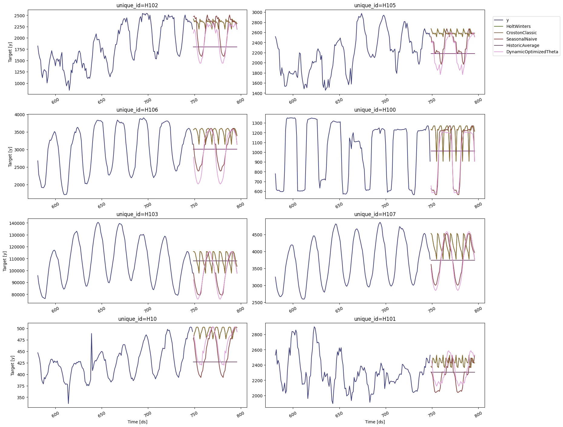
Plot the results of 8 random series using the `StatsForecast.plot`
method.
```python theme={null}
sf.plot(Y_df,forecasts_df)
```
## Train multiple models for many series
StatsForecast can train many models on many time series efficiently.
Start by importing and instantiating the desired models. StatsForecast
offers a wide variety of models grouped in the following categories:
* **Auto Forecast:** Automatic forecasting tools search for the best
parameters and select the best possible model for a series of time
series. These tools are useful for large collections of univariate
time series. Includes automatic versions of: Arima, ETS, Theta, CES.
* **Exponential Smoothing:** Uses a weighted average of all past
observations where the weights decrease exponentially into the past.
Suitable for data with no clear trend or seasonality. Examples: SES,
Holt’s Winters, SSO.
* **Benchmark models:** classical models for establishing baselines.
Examples: Mean, Naive, Random Walk
* **Intermittent or Sparse models:** suited for series with very few
non-zero observations. Examples: CROSTON, ADIDA, IMAPA
* **Multiple Seasonalities:** suited for signals with more than one
clear seasonality. Useful for low-frequency data like electricity
and logs. Examples: MSTL.
* **Theta Models:** fit two theta lines to a deseasonalized time
series, using different techniques to obtain and combine the two
theta lines to produce the final forecasts. Examples: Theta,
DynamicTheta
Here you can check the complete list of
[models](../../src/core/models_intro.html).
For this example we will use:
* `AutoARIMA`: Automatically selects the best ARIMA (AutoRegressive
Integrated Moving Average) model using an information criterion.
Ref: `AutoARIMA`.
* `HoltWinters`: triple exponential smoothing, Holt-Winters’ method is
an extension of exponential smoothing for series that contain both
trend and seasonality. Ref: `HoltWinters`
* `SeasonalNaive`: Memory Efficient Seasonal Naive predictions. Ref:
`SeasonalNaive`
* `HistoricAverage`: arithmetic mean. Ref: `HistoricAverage`.
* `DynamicOptimizedTheta`: The theta family of models has been shown
to perform well in various datasets such as M3. Models the
deseasonalized time series. Ref: `DynamicOptimizedTheta`.
Import and instantiate the models. Setting the `season_length` argument
is sometimes tricky. This article on [Seasonal
periods](https://robjhyndman.com/hyndsight/seasonal-periods/)) by the
master, Rob Hyndmann, can be useful.
```python theme={null}
from statsforecast.models import (
HoltWinters,
CrostonClassic as Croston,
HistoricAverage,
DynamicOptimizedTheta as DOT,
SeasonalNaive
)
```
```python theme={null}
# Create a list of models and instantiation parameters
models = [
HoltWinters(),
Croston(),
SeasonalNaive(season_length=24),
HistoricAverage(),
DOT(season_length=24)
]
```
We fit the models by instantiating a new `StatsForecast` object with the
following parameters:
* `models`: a list of models. Select the models you want from
[models](../../src/core/models_intro.html) and import them.
* `freq`: a string indicating the frequency of the data. (See [panda’s
available
frequencies](https://pandas.pydata.org/pandas-docs/stable/user_guide/timeseries.html#offset-aliases).)
This is also available with Polars.
* `n_jobs`: int, number of jobs used in the parallel processing, use
-1 for all cores.
* `fallback_model`: a model to be used if a model fails.
Any settings are passed into the constructor. Then you call its fit
method and pass in the historical data frame.
```python theme={null}
# Instantiate StatsForecast class as sf
sf = StatsForecast(
models=models,
freq=1,
n_jobs=-1,
fallback_model=SeasonalNaive(season_length=7),
verbose=True,
)
```
The `forecast` method takes two arguments: forecasts next `h` (horizon)
and `level`.
* `h` (int): represents the forecast h steps into the future. In this
case, 12 months ahead.
* `level` (list of floats): this optional parameter is used for
probabilistic forecasting. Set the `level` (or confidence
percentile) of your prediction interval. For example, `level=[90]`
means that the model expects the real value to be inside that
interval 90% of the times.
The forecast object here is a new data frame that includes a column with
the name of the model and the y hat values, as well as columns for the
uncertainty intervals. Depending on your computer, this step should take
around 1min. (If you want to speed things up to a couple of seconds,
remove the AutoModels like ARIMA and Theta)
> **Note**
>
> The `forecast` method is compatible with distributed clusters, so it
> does not store any model parameters. If you want to store parameters
> for every model you can use the `fit` and `predict` methods. However,
> those methods are not defined for distributed engines like Spark, Ray
> or Dask.
```python theme={null}
forecasts_df = sf.forecast(df=Y_df, h=48, level=[90])
forecasts_df.head()
```
```text theme={null}
Forecast: 100%|██████████| 10/10 [Elapsed: 00:03]
```
| unique\_id | ds | HoltWinters | HoltWinters-lo-90 | HoltWinters-hi-90 | CrostonClassic | CrostonClassic-lo-90 | CrostonClassic-hi-90 | SeasonalNaive | SeasonalNaive-lo-90 | SeasonalNaive-hi-90 | HistoricAverage | HistoricAverage-lo-90 | HistoricAverage-hi-90 | DynamicOptimizedTheta | DynamicOptimizedTheta-lo-90 | DynamicOptimizedTheta-hi-90 |
| ---------- | --- | ----------- | ----------------- | ----------------- | -------------- | -------------------- | -------------------- | ------------- | ------------------- | ------------------- | --------------- | --------------------- | --------------------- | --------------------- | --------------------------- | --------------------------- |
| str | i64 | f64 | f64 | f64 | f64 | f64 | f64 | f64 | f64 | f64 | f64 | f64 | f64 | f64 | f64 | f64 |
| "H1" | 749 | 829.0 | 422.549268 | 1235.450732 | 829.0 | 422.549268 | 1235.450732 | 635.0 | 566.036734 | 703.963266 | 660.982143 | 398.037761 | 923.926524 | 592.701851 | 577.67728 | 611.652639 |
| "H1" | 750 | 807.0 | 400.549268 | 1213.450732 | 807.0 | 400.549268 | 1213.450732 | 572.0 | 503.036734 | 640.963266 | 660.982143 | 398.037761 | 923.926524 | 525.589117 | 505.449755 | 546.621805 |
| "H1" | 751 | 785.0 | 378.549268 | 1191.450732 | 785.0 | 378.549268 | 1191.450732 | 532.0 | 463.036734 | 600.963266 | 660.982143 | 398.037761 | 923.926524 | 489.251814 | 462.072871 | 512.424116 |
| "H1" | 752 | 756.0 | 349.549268 | 1162.450732 | 756.0 | 349.549268 | 1162.450732 | 493.0 | 424.036734 | 561.963266 | 660.982143 | 398.037761 | 923.926524 | 456.195032 | 430.554302 | 478.260963 |
| "H1" | 753 | 719.0 | 312.549268 | 1125.450732 | 719.0 | 312.549268 | 1125.450732 | 477.0 | 408.036734 | 545.963266 | 660.982143 | 398.037761 | 923.926524 | 436.290514 | 411.051232 | 461.815932 |
Plot the results of 8 random series using the `StatsForecast.plot`
method.
```python theme={null}
sf.plot(Y_df,forecasts_df)
```
 The `StatsForecast.plot` allows for further customization. For example,
plot the results of the different models and unique ids.
```python theme={null}
# Plot to unique_ids and some selected models
sf.plot(Y_df, forecasts_df, models=["HoltWinters","DynamicOptimizedTheta"], unique_ids=["H10", "H105"], level=[90])
```
The `StatsForecast.plot` allows for further customization. For example,
plot the results of the different models and unique ids.
```python theme={null}
# Plot to unique_ids and some selected models
sf.plot(Y_df, forecasts_df, models=["HoltWinters","DynamicOptimizedTheta"], unique_ids=["H10", "H105"], level=[90])
```
 ```python theme={null}
# Explore other models
sf.plot(Y_df, forecasts_df, models=["SeasonalNaive"], unique_ids=["H10", "H105"], level=[90])
```
```python theme={null}
# Explore other models
sf.plot(Y_df, forecasts_df, models=["SeasonalNaive"], unique_ids=["H10", "H105"], level=[90])
```
 ## Evaluate the model’s performance
In previous steps, we’ve taken our historical data to predict the
future. However, to assess its accuracy we would also like to know how
the model would have performed in the past. To assess the accuracy and
robustness of your models on your data perform Cross-Validation.
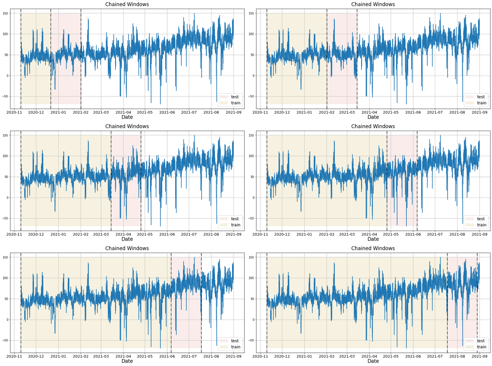
With time series data, **Cross Validation** is done by defining a
sliding window across the historical data and predicting the period
following it. This form of cross-validation allows us to arrive at a
better estimation of our model’s predictive abilities across a wider
range of temporal instances while also keeping the data in the training
set contiguous as is required by our models.
The following graph depicts such a Cross Validation Strategy:
Cross-validation of time series models is considered a best practice but
most implementations are very slow. The statsforecast library implements
cross-validation as a distributed operation, making the process less
time-consuming to perform. If you have big datasets you can also perform
Cross Validation in a distributed cluster using Ray, Dask or Spark.
In this case, we want to evaluate the performance of each model for the
last 2 days (n\_windows=2), forecasting every second day (step\_size=48).
Depending on your computer, this step should take around 1 min.
> **Tip**
>
> Setting `n_windows=1` mirrors a traditional train-test split with our
> historical data serving as the training set and the last 48 hours
> serving as the testing set.
The `cross_validation` method from the `StatsForecast` class takes the
following arguments.
* `df`: training data frame
* `h` (int): represents h steps into the future that are being
forecasted. In this case, 24 hours ahead.
* `step_size` (int): step size between each window. In other words:
how often do you want to run the forecasting processes.
* `n_windows`(int): number of windows used for cross validation. In
other words: what number of forecasting processes in the past do you
want to evaluate.
```python theme={null}
cv_df = sf.cross_validation(
df=Y_df,
h=24,
step_size=24,
n_windows=2
)
```
```text theme={null}
Cross Validation Time Series 1: 100%|██████████| 2/2 [00:00<00:00, 2.02it/s]
Cross Validation Time Series 1: 100%|██████████| 2/2 [00:00<00:00, 2.02it/s]
Cross Validation Time Series 1: 100%|██████████| 2/2 [00:00<00:00, 2.26it/s]
Cross Validation Time Series 1: 100%|██████████| 2/2 [00:00<00:00, 2.76it/s]
Cross Validation Time Series 1: 100%|██████████| 2/2 [00:00<00:00, 2.25it/s]
Cross Validation Time Series 1: 100%|██████████| 2/2 [00:00<00:00, 2.78it/s]
Cross Validation Time Series 1: 100%|██████████| 2/2 [00:00<00:00, 3.20it/s]
Cross Validation Time Series 1: 100%|██████████| 2/2 [00:00<00:00, 4.14it/s]
Cross Validation Time Series 1: 100%|██████████| 2/2 [00:00<00:00, 4.11it/s]
Cross Validation Time Series 1: 100%|██████████| 2/2 [00:00<00:00, 4.75it/s]
```
The `cv_df` object is a new data frame that includes the following
columns:
* `unique_id`: series identifier
* `ds`: datestamp or temporal index
* `cutoff`: the last datestamp or temporal index for the `n_windows.`
If `n_windows=1`, then one unique cutoff value, if `n_windows=2`
then two unique cutoff values.
* `y`: true value
* `"model"`: columns with the model’s name and fitted value.
```python theme={null}
cv_df.head()
```
| unique\_id | ds | cutoff | y | HoltWinters | CrostonClassic | SeasonalNaive | HistoricAverage | DynamicOptimizedTheta |
| ---------- | --- | ------ | ----- | ----------- | -------------- | ------------- | --------------- | --------------------- |
| str | i64 | i64 | f64 | f64 | f64 | f64 | f64 | f64 |
| "H1" | 701 | 700 | 619.0 | 847.0 | 742.668748 | 691.0 | 661.675 | 612.767525 |
| "H1" | 702 | 700 | 565.0 | 820.0 | 742.668748 | 618.0 | 661.675 | 536.846296 |
| "H1" | 703 | 700 | 532.0 | 790.0 | 742.668748 | 563.0 | 661.675 | 497.824302 |
| "H1" | 704 | 700 | 495.0 | 784.0 | 742.668748 | 529.0 | 661.675 | 464.723235 |
| "H1" | 705 | 700 | 481.0 | 752.0 | 742.668748 | 504.0 | 661.675 | 440.972351 |
Next, we will evaluate the performance of every model for every series
using common error metrics like Mean Absolute Error (MAE) or Mean Square
Error (MSE) Define a utility function to evaluate different error
metrics for the cross validation data frame.
First import the desired error metrics from `utilsforecast.losses`. Then
define a utility function that takes a cross-validation data frame as a
metric and returns an evaluation data frame with the average of the
error metric for every unique id and fitted model and all cutoffs.
```python theme={null}
from utilsforecast.evaluation import evaluate
from utilsforecast.losses import mse
```
```python theme={null}
def evaluate_cv(df, metric):
models = [c for c in df.columns if c not in ('unique_id', 'ds', 'cutoff', 'y')]
evals = evaluate(df, metrics=[metric], models=models)
evals = evals.drop('metric')
pos2model = dict(enumerate(models))
return evals.with_columns(
best_model=pl.concat_list(models).list.arg_min().replace_strict(pos2model)
)
```
> **Warning**
>
> You can also use Mean Average Percentage Error (MAPE), however for
> granular forecasts, MAPE values are extremely [hard to
> judge](https://blog.blueyonder.com/mean-absolute-percentage-error-mape-has-served-its-duty-and-should-now-retire/)
> and not useful to assess forecasting quality.
Create the data frame with the results of the evaluation of your
cross-validation data frame using a Mean Squared Error metric.
```python theme={null}
evaluation_df = evaluate_cv(cv_df, mse)
evaluation_df.head()
```
| unique\_id | cutoff | HoltWinters | CrostonClassic | SeasonalNaive | HistoricAverage | DynamicOptimizedTheta | best\_model |
| ---------- | ------ | ------------- | -------------- | ------------- | --------------- | --------------------- | ---------------- |
| str | i64 | f64 | f64 | f64 | f64 | f64 | str |
| "H1" | 700 | 38009.958333 | 28751.156365 | 1517.5 | 23823.193125 | 1595.491947 | "SeasonalNaive" |
| "H10" | 700 | 2617.458333 | 1429.094499 | 89.375 | 1833.382222 | 397.616596 | "SeasonalNaive" |
| "H100" | 700 | 104198.5 | 80556.697053 | 8313.25 | 71869.350278 | 28936.963781 | "SeasonalNaive" |
| "H101" | 700 | 19922.958333 | 6907.766752 | 13607.708333 | 9870.140347 | 107823.332195 | "CrostonClassic" |
| "H102" | 700 | 264394.791667 | 144611.993865 | 9206.166667 | 350475.255208 | 32221.37975 | "SeasonalNaive" |
Create a summary table with a model column and the number of series
where that model performs best. In this case, the Arima and Seasonal
Naive are the best models for 10 series and the Theta model should be
used for two.
```python theme={null}
evaluation_df['best_model'].value_counts()
```
| best\_model | count |
| ----------------------- | ----- |
| str | u32 |
| "SeasonalNaive" | 11 |
| "CrostonClassic" | 1 |
| "DynamicOptimizedTheta" | 8 |
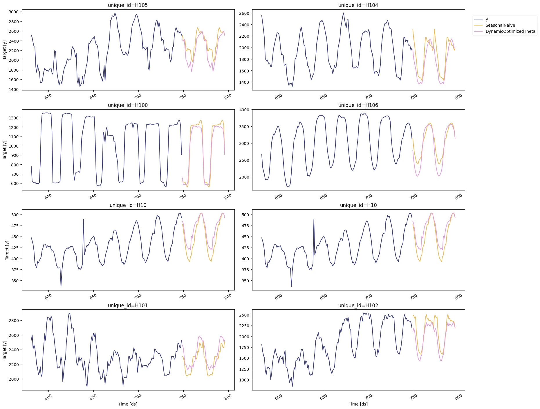
You can further explore your results by plotting the unique\_ids where a
specific model wins.
```python theme={null}
seasonal_ids = evaluation_df.filter(pl.col('best_model') == 'SeasonalNaive')['unique_id']
sf.plot(Y_df,forecasts_df, unique_ids=seasonal_ids, models=["SeasonalNaive","DynamicOptimizedTheta"])
```
## Evaluate the model’s performance
In previous steps, we’ve taken our historical data to predict the
future. However, to assess its accuracy we would also like to know how
the model would have performed in the past. To assess the accuracy and
robustness of your models on your data perform Cross-Validation.
With time series data, **Cross Validation** is done by defining a
sliding window across the historical data and predicting the period
following it. This form of cross-validation allows us to arrive at a
better estimation of our model’s predictive abilities across a wider
range of temporal instances while also keeping the data in the training
set contiguous as is required by our models.
The following graph depicts such a Cross Validation Strategy:

Cross-validation of time series models is considered a best practice but
most implementations are very slow. The statsforecast library implements
cross-validation as a distributed operation, making the process less
time-consuming to perform. If you have big datasets you can also perform
Cross Validation in a distributed cluster using Ray, Dask or Spark.
In this case, we want to evaluate the performance of each model for the
last 2 days (n\_windows=2), forecasting every second day (step\_size=48).
Depending on your computer, this step should take around 1 min.
> **Tip**
>
> Setting `n_windows=1` mirrors a traditional train-test split with our
> historical data serving as the training set and the last 48 hours
> serving as the testing set.
The `cross_validation` method from the `StatsForecast` class takes the
following arguments.
* `df`: training data frame
* `h` (int): represents h steps into the future that are being
forecasted. In this case, 24 hours ahead.
* `step_size` (int): step size between each window. In other words:
how often do you want to run the forecasting processes.
* `n_windows`(int): number of windows used for cross validation. In
other words: what number of forecasting processes in the past do you
want to evaluate.
```python theme={null}
cv_df = sf.cross_validation(
df=Y_df,
h=24,
step_size=24,
n_windows=2
)
```
```text theme={null}
Cross Validation Time Series 1: 100%|██████████| 2/2 [00:00<00:00, 2.02it/s]
Cross Validation Time Series 1: 100%|██████████| 2/2 [00:00<00:00, 2.02it/s]
Cross Validation Time Series 1: 100%|██████████| 2/2 [00:00<00:00, 2.26it/s]
Cross Validation Time Series 1: 100%|██████████| 2/2 [00:00<00:00, 2.76it/s]
Cross Validation Time Series 1: 100%|██████████| 2/2 [00:00<00:00, 2.25it/s]
Cross Validation Time Series 1: 100%|██████████| 2/2 [00:00<00:00, 2.78it/s]
Cross Validation Time Series 1: 100%|██████████| 2/2 [00:00<00:00, 3.20it/s]
Cross Validation Time Series 1: 100%|██████████| 2/2 [00:00<00:00, 4.14it/s]
Cross Validation Time Series 1: 100%|██████████| 2/2 [00:00<00:00, 4.11it/s]
Cross Validation Time Series 1: 100%|██████████| 2/2 [00:00<00:00, 4.75it/s]
```
The `cv_df` object is a new data frame that includes the following
columns:
* `unique_id`: series identifier
* `ds`: datestamp or temporal index
* `cutoff`: the last datestamp or temporal index for the `n_windows.`
If `n_windows=1`, then one unique cutoff value, if `n_windows=2`
then two unique cutoff values.
* `y`: true value
* `"model"`: columns with the model’s name and fitted value.
```python theme={null}
cv_df.head()
```
| unique\_id | ds | cutoff | y | HoltWinters | CrostonClassic | SeasonalNaive | HistoricAverage | DynamicOptimizedTheta |
| ---------- | --- | ------ | ----- | ----------- | -------------- | ------------- | --------------- | --------------------- |
| str | i64 | i64 | f64 | f64 | f64 | f64 | f64 | f64 |
| "H1" | 701 | 700 | 619.0 | 847.0 | 742.668748 | 691.0 | 661.675 | 612.767525 |
| "H1" | 702 | 700 | 565.0 | 820.0 | 742.668748 | 618.0 | 661.675 | 536.846296 |
| "H1" | 703 | 700 | 532.0 | 790.0 | 742.668748 | 563.0 | 661.675 | 497.824302 |
| "H1" | 704 | 700 | 495.0 | 784.0 | 742.668748 | 529.0 | 661.675 | 464.723235 |
| "H1" | 705 | 700 | 481.0 | 752.0 | 742.668748 | 504.0 | 661.675 | 440.972351 |
Next, we will evaluate the performance of every model for every series
using common error metrics like Mean Absolute Error (MAE) or Mean Square
Error (MSE) Define a utility function to evaluate different error
metrics for the cross validation data frame.
First import the desired error metrics from `utilsforecast.losses`. Then
define a utility function that takes a cross-validation data frame as a
metric and returns an evaluation data frame with the average of the
error metric for every unique id and fitted model and all cutoffs.
```python theme={null}
from utilsforecast.evaluation import evaluate
from utilsforecast.losses import mse
```
```python theme={null}
def evaluate_cv(df, metric):
models = [c for c in df.columns if c not in ('unique_id', 'ds', 'cutoff', 'y')]
evals = evaluate(df, metrics=[metric], models=models)
evals = evals.drop('metric')
pos2model = dict(enumerate(models))
return evals.with_columns(
best_model=pl.concat_list(models).list.arg_min().replace_strict(pos2model)
)
```
> **Warning**
>
> You can also use Mean Average Percentage Error (MAPE), however for
> granular forecasts, MAPE values are extremely [hard to
> judge](https://blog.blueyonder.com/mean-absolute-percentage-error-mape-has-served-its-duty-and-should-now-retire/)
> and not useful to assess forecasting quality.
Create the data frame with the results of the evaluation of your
cross-validation data frame using a Mean Squared Error metric.
```python theme={null}
evaluation_df = evaluate_cv(cv_df, mse)
evaluation_df.head()
```
| unique\_id | cutoff | HoltWinters | CrostonClassic | SeasonalNaive | HistoricAverage | DynamicOptimizedTheta | best\_model |
| ---------- | ------ | ------------- | -------------- | ------------- | --------------- | --------------------- | ---------------- |
| str | i64 | f64 | f64 | f64 | f64 | f64 | str |
| "H1" | 700 | 38009.958333 | 28751.156365 | 1517.5 | 23823.193125 | 1595.491947 | "SeasonalNaive" |
| "H10" | 700 | 2617.458333 | 1429.094499 | 89.375 | 1833.382222 | 397.616596 | "SeasonalNaive" |
| "H100" | 700 | 104198.5 | 80556.697053 | 8313.25 | 71869.350278 | 28936.963781 | "SeasonalNaive" |
| "H101" | 700 | 19922.958333 | 6907.766752 | 13607.708333 | 9870.140347 | 107823.332195 | "CrostonClassic" |
| "H102" | 700 | 264394.791667 | 144611.993865 | 9206.166667 | 350475.255208 | 32221.37975 | "SeasonalNaive" |
Create a summary table with a model column and the number of series
where that model performs best. In this case, the Arima and Seasonal
Naive are the best models for 10 series and the Theta model should be
used for two.
```python theme={null}
evaluation_df['best_model'].value_counts()
```
| best\_model | count |
| ----------------------- | ----- |
| str | u32 |
| "SeasonalNaive" | 11 |
| "CrostonClassic" | 1 |
| "DynamicOptimizedTheta" | 8 |
You can further explore your results by plotting the unique\_ids where a
specific model wins.
```python theme={null}
seasonal_ids = evaluation_df.filter(pl.col('best_model') == 'SeasonalNaive')['unique_id']
sf.plot(Y_df,forecasts_df, unique_ids=seasonal_ids, models=["SeasonalNaive","DynamicOptimizedTheta"])
```
 ## Select the best model for every unique series
Define a utility function that takes your forecast’s data frame with the
predictions and the evaluation data frame and returns a data frame with
the best possible forecast for every unique\_id.
```python theme={null}
def get_best_model_forecast(forecasts_df, evaluation_df):
models = {
c.replace('-lo-90', '').replace('-hi-90', '')
for c in forecasts_df.columns
if c not in ('unique_id', 'ds')
}
model2pos = {m: i for i, m in enumerate(models)}
with_best = forecasts_df.join(evaluation_df[['unique_id', 'best_model']], on='unique_id')
return with_best.select(
'unique_id',
'ds',
*[
(
pl.concat_list([f'{m}{suffix}' for m in models])
.list.get(pl.col('best_model').replace_strict(model2pos))
.alias(f'best_model{suffix}')
)
for suffix in ('', '-lo-90', '-hi-90')
]
)
```
Create your production-ready data frame with the best forecast for every
unique\_id.
```python theme={null}
prod_forecasts_df = get_best_model_forecast(forecasts_df, evaluation_df)
prod_forecasts_df.head()
```
| unique\_id | ds | best\_model | best\_model-lo-90 | best\_model-hi-90 |
| ---------- | --- | ----------- | ----------------- | ----------------- |
| str | i64 | f64 | f64 | f64 |
| "H1" | 749 | 635.0 | 566.036734 | 703.963266 |
| "H1" | 749 | 592.701851 | 577.67728 | 611.652639 |
| "H1" | 750 | 572.0 | 503.036734 | 640.963266 |
| "H1" | 750 | 525.589117 | 505.449755 | 546.621805 |
| "H1" | 751 | 532.0 | 463.036734 | 600.963266 |
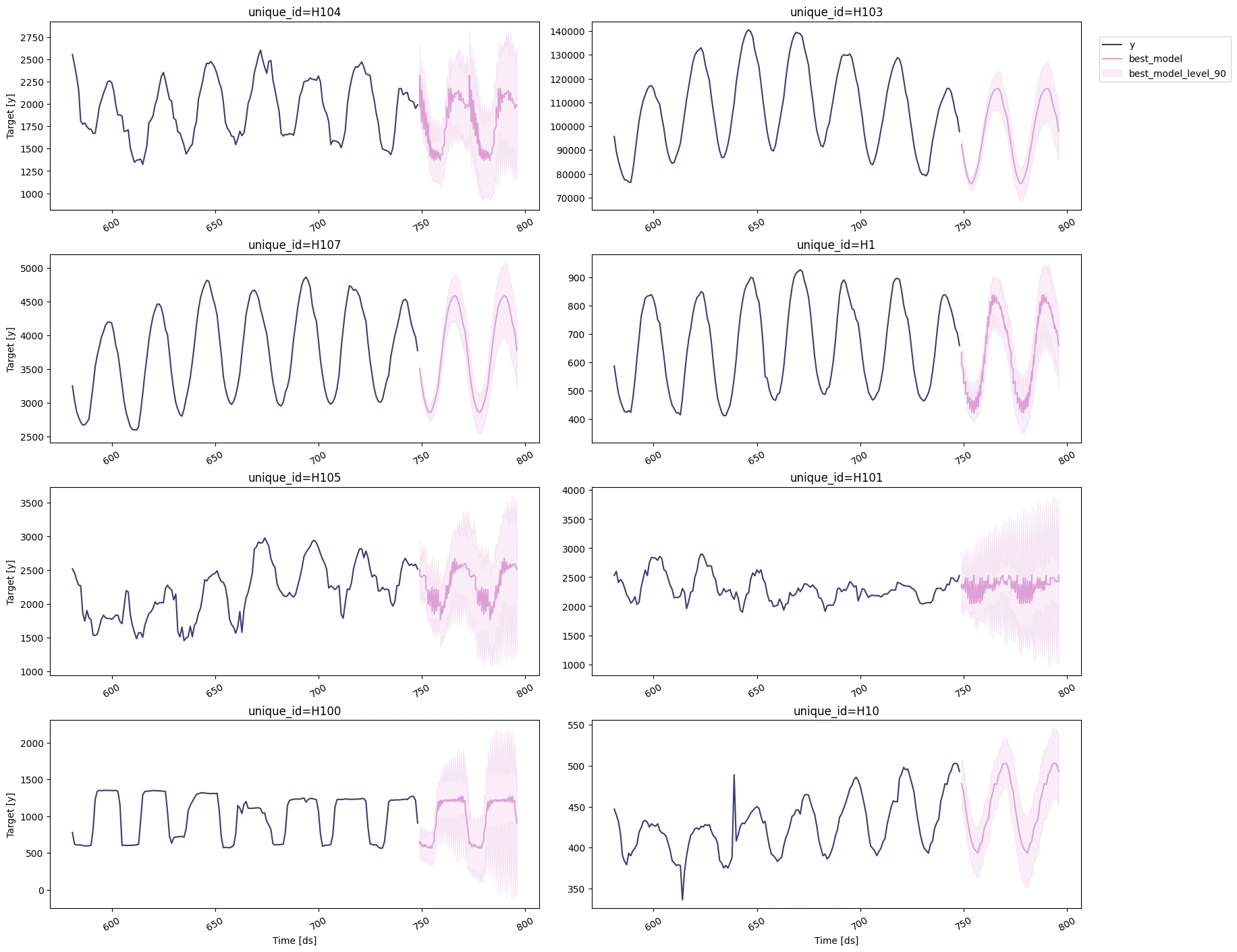
Plot the results.
```python theme={null}
sf.plot(Y_df, prod_forecasts_df, level=[90])
```
## Select the best model for every unique series
Define a utility function that takes your forecast’s data frame with the
predictions and the evaluation data frame and returns a data frame with
the best possible forecast for every unique\_id.
```python theme={null}
def get_best_model_forecast(forecasts_df, evaluation_df):
models = {
c.replace('-lo-90', '').replace('-hi-90', '')
for c in forecasts_df.columns
if c not in ('unique_id', 'ds')
}
model2pos = {m: i for i, m in enumerate(models)}
with_best = forecasts_df.join(evaluation_df[['unique_id', 'best_model']], on='unique_id')
return with_best.select(
'unique_id',
'ds',
*[
(
pl.concat_list([f'{m}{suffix}' for m in models])
.list.get(pl.col('best_model').replace_strict(model2pos))
.alias(f'best_model{suffix}')
)
for suffix in ('', '-lo-90', '-hi-90')
]
)
```
Create your production-ready data frame with the best forecast for every
unique\_id.
```python theme={null}
prod_forecasts_df = get_best_model_forecast(forecasts_df, evaluation_df)
prod_forecasts_df.head()
```
| unique\_id | ds | best\_model | best\_model-lo-90 | best\_model-hi-90 |
| ---------- | --- | ----------- | ----------------- | ----------------- |
| str | i64 | f64 | f64 | f64 |
| "H1" | 749 | 635.0 | 566.036734 | 703.963266 |
| "H1" | 749 | 592.701851 | 577.67728 | 611.652639 |
| "H1" | 750 | 572.0 | 503.036734 | 640.963266 |
| "H1" | 750 | 525.589117 | 505.449755 | 546.621805 |
| "H1" | 751 | 532.0 | 463.036734 | 600.963266 |
Plot the results.
```python theme={null}
sf.plot(Y_df, prod_forecasts_df, level=[90])
```