> ## Documentation Index
> Fetch the complete documentation index at: https://nixtlaverse.nixtla.io/llms.txt
> Use this file to discover all available pages before exploring further.
# AutoARIMA Comparison (Prophet and pmdarima)
 ## Motivation
The `AutoARIMA` model is widely used to forecast time series in
production and as a benchmark. However, the python implementation
(`pmdarima`) is so slow that prevent data scientist practioners from
quickly iterating and deploying `AutoARIMA` in production for a large
number of time series. In this notebook we present Nixtla’s `AutoARIMA`
based on the R implementation (developed by Rob Hyndman) and optimized
using `numba`.
## Example
### Libraries
```python theme={null}
%%capture
# !pip install statsforecast prophet statsmodels sklearn matplotlib pmdarima
```
```python theme={null}
import logging
import os
import random
import time
import warnings
warnings.filterwarnings("ignore")
from itertools import product
from multiprocessing import cpu_count, Pool # for prophet
import matplotlib.pyplot as plt
import numpy as np
import pandas as pd
from pmdarima import auto_arima as auto_arima_p
from prophet import Prophet
from statsforecast import StatsForecast
from statsforecast.models import AutoARIMA, _TS
from statsmodels.graphics.tsaplots import plot_acf
from sklearn.model_selection import ParameterGrid
from utilsforecast.plotting import plot_series
```
#### Useful functions
```python theme={null}
def plot_autocorrelation_grid(df_train):
fig, axes = plt.subplots(4, 2, figsize = (24, 14))
unique_ids = df_train['unique_id'].unique()
assert len(unique_ids) >= 8, "Must provide at least 8 ts"
unique_ids = random.sample(list(unique_ids), k=8)
for uid, (idx, idy) in zip(unique_ids, product(range(4), range(2))):
train_uid = df_train.query('unique_id == @uid')
plot_acf(train_uid['y'].values, ax=axes[idx, idy],
title=f'ACF M4 Hourly {uid}')
axes[idx, idy].set_xlabel('Timestamp [t]')
axes[idx, idy].set_ylabel('Autocorrelation')
fig.subplots_adjust(hspace=0.5)
plt.show()
```
### Data
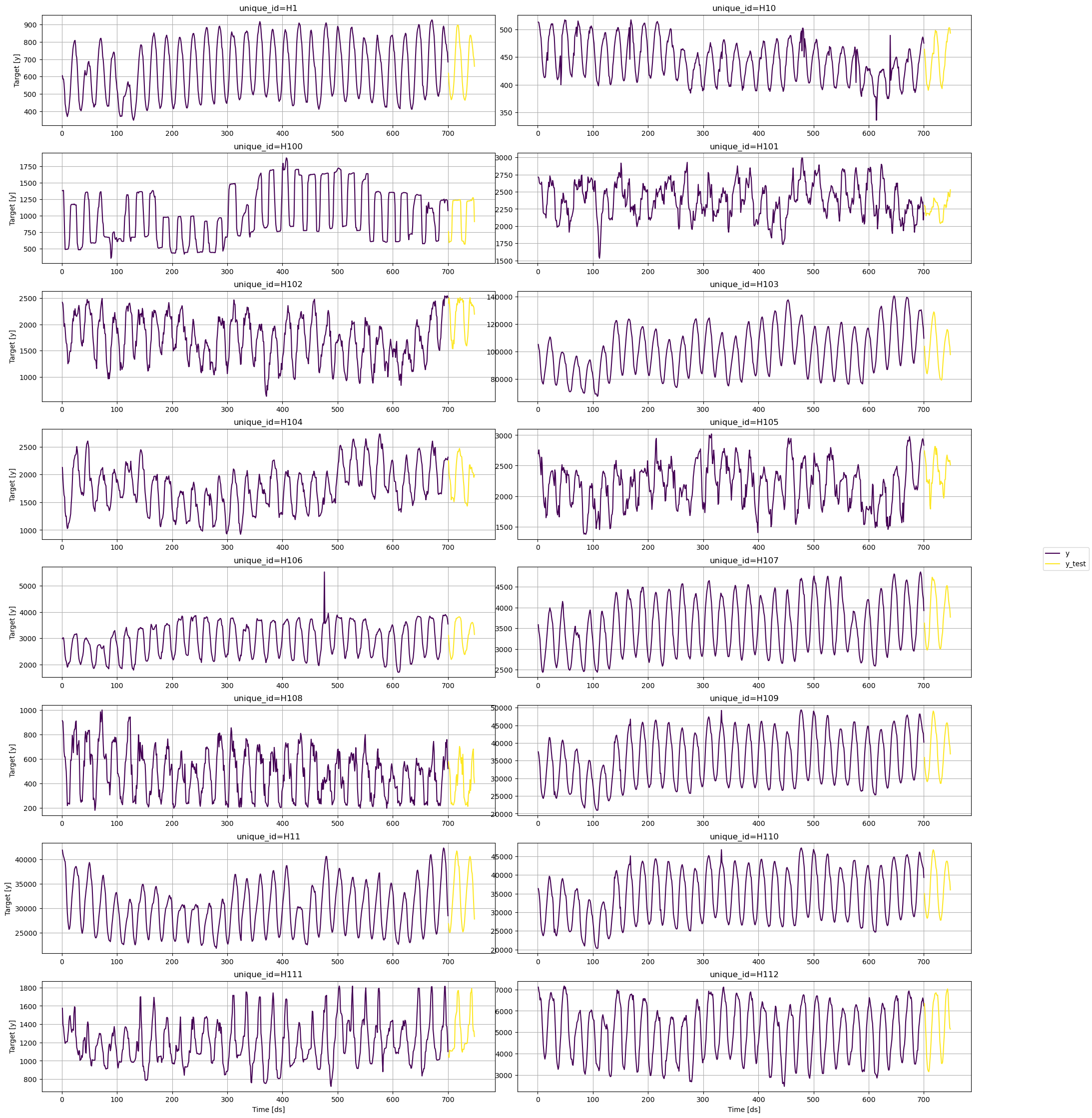
For testing purposes, we will use the Hourly dataset from the M4
competition.
```python theme={null}
train = pd.read_csv('https://auto-arima-results.s3.amazonaws.com/M4-Hourly.csv')
test = pd.read_csv('https://auto-arima-results.s3.amazonaws.com/M4-Hourly-test.csv').rename(columns={'y': 'y_test'})
```
In this example we will use a subset of the data to avoid waiting too
long. You can modify the number of series if you want.
```python theme={null}
n_series = 16
uids = train['unique_id'].unique()[:n_series]
train = train.query('unique_id in @uids')
test = test.query('unique_id in @uids')
```
```python theme={null}
plot_series(train, test, max_ids=n_series)
```
## Motivation
The `AutoARIMA` model is widely used to forecast time series in
production and as a benchmark. However, the python implementation
(`pmdarima`) is so slow that prevent data scientist practioners from
quickly iterating and deploying `AutoARIMA` in production for a large
number of time series. In this notebook we present Nixtla’s `AutoARIMA`
based on the R implementation (developed by Rob Hyndman) and optimized
using `numba`.
## Example
### Libraries
```python theme={null}
%%capture
# !pip install statsforecast prophet statsmodels sklearn matplotlib pmdarima
```
```python theme={null}
import logging
import os
import random
import time
import warnings
warnings.filterwarnings("ignore")
from itertools import product
from multiprocessing import cpu_count, Pool # for prophet
import matplotlib.pyplot as plt
import numpy as np
import pandas as pd
from pmdarima import auto_arima as auto_arima_p
from prophet import Prophet
from statsforecast import StatsForecast
from statsforecast.models import AutoARIMA, _TS
from statsmodels.graphics.tsaplots import plot_acf
from sklearn.model_selection import ParameterGrid
from utilsforecast.plotting import plot_series
```
#### Useful functions
```python theme={null}
def plot_autocorrelation_grid(df_train):
fig, axes = plt.subplots(4, 2, figsize = (24, 14))
unique_ids = df_train['unique_id'].unique()
assert len(unique_ids) >= 8, "Must provide at least 8 ts"
unique_ids = random.sample(list(unique_ids), k=8)
for uid, (idx, idy) in zip(unique_ids, product(range(4), range(2))):
train_uid = df_train.query('unique_id == @uid')
plot_acf(train_uid['y'].values, ax=axes[idx, idy],
title=f'ACF M4 Hourly {uid}')
axes[idx, idy].set_xlabel('Timestamp [t]')
axes[idx, idy].set_ylabel('Autocorrelation')
fig.subplots_adjust(hspace=0.5)
plt.show()
```
### Data
For testing purposes, we will use the Hourly dataset from the M4
competition.
```python theme={null}
train = pd.read_csv('https://auto-arima-results.s3.amazonaws.com/M4-Hourly.csv')
test = pd.read_csv('https://auto-arima-results.s3.amazonaws.com/M4-Hourly-test.csv').rename(columns={'y': 'y_test'})
```
In this example we will use a subset of the data to avoid waiting too
long. You can modify the number of series if you want.
```python theme={null}
n_series = 16
uids = train['unique_id'].unique()[:n_series]
train = train.query('unique_id in @uids')
test = test.query('unique_id in @uids')
```
```python theme={null}
plot_series(train, test, max_ids=n_series)
```
 Would an autorregresive model be the right choice for our data? There is
no doubt that we observe seasonal periods. The autocorrelation function
(`acf`) can help us to answer the question. Intuitively, we have to
observe a decreasing correlation to opt for an AR model.
```python theme={null}
plot_autocorrelation_grid(train)
```
Would an autorregresive model be the right choice for our data? There is
no doubt that we observe seasonal periods. The autocorrelation function
(`acf`) can help us to answer the question. Intuitively, we have to
observe a decreasing correlation to opt for an AR model.
```python theme={null}
plot_autocorrelation_grid(train)
```
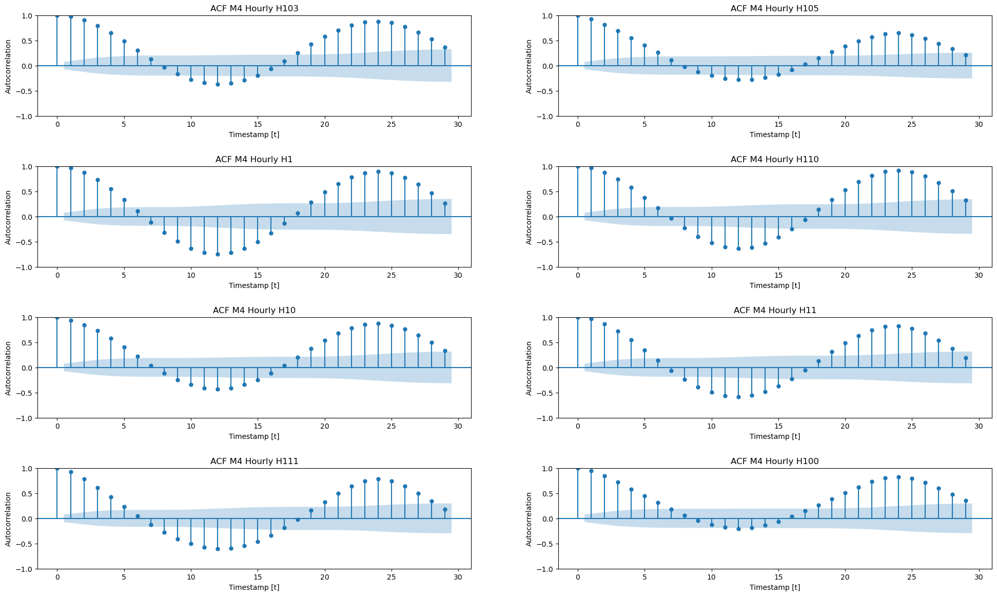 Thus, we observe a high autocorrelation for previous lags and also for
the seasonal lags. Therefore, we will let `auto_arima` to handle our
data.
### Training and forecasting
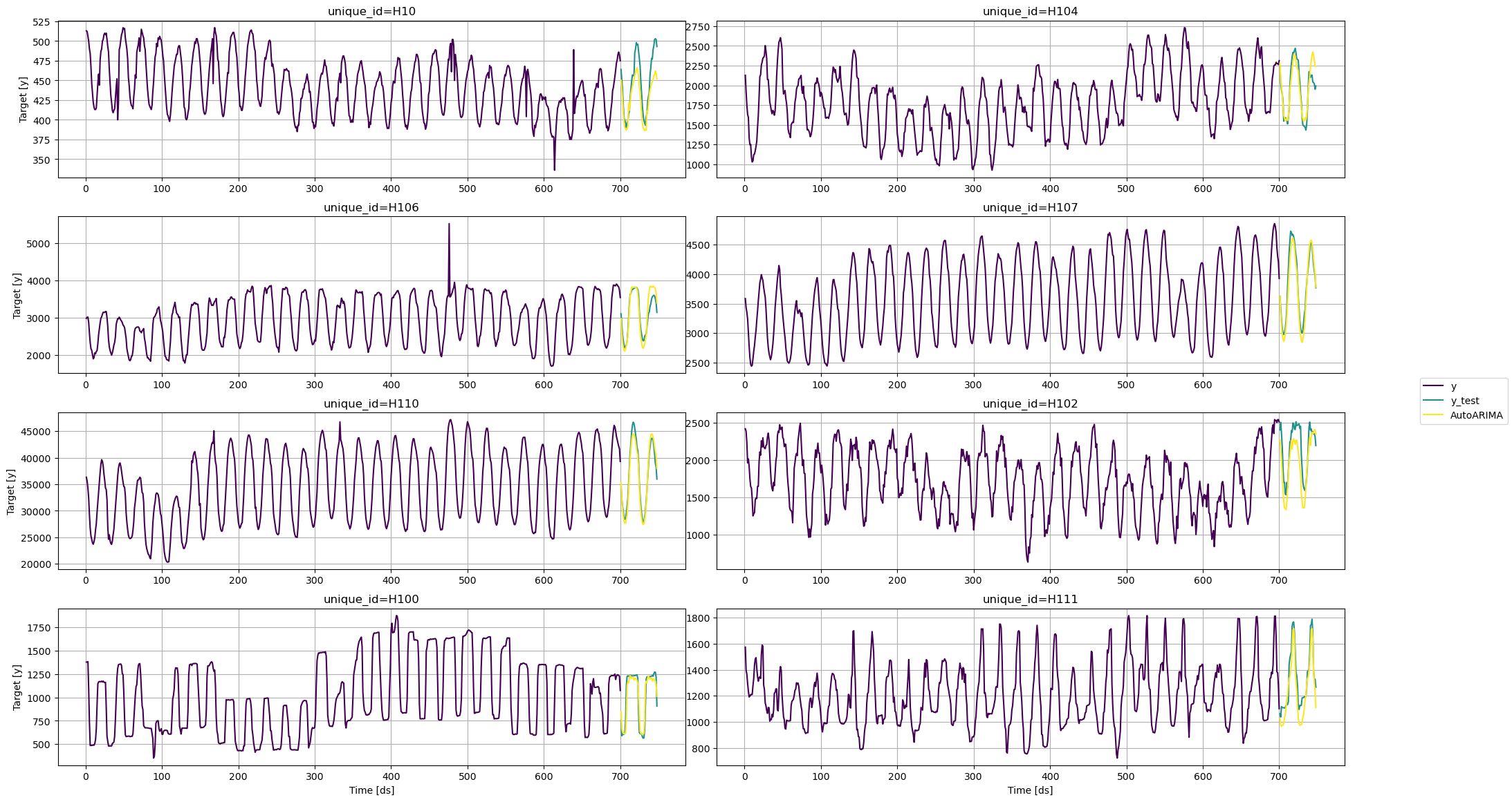
`StatsForecast` receives a list of models to fit each time series. Since
we are dealing with Hourly data, it would be benefitial to use 24 as
seasonality.
```python theme={null}
?AutoARIMA
```
```text theme={null}
Init signature:
AutoARIMA(
d: Optional[int] = None,
D: Optional[int] = None,
max_p: int = 5,
max_q: int = 5,
max_P: int = 2,
max_Q: int = 2,
max_order: int = 5,
max_d: int = 2,
max_D: int = 1,
start_p: int = 2,
start_q: int = 2,
start_P: int = 1,
start_Q: int = 1,
stationary: bool = False,
seasonal: bool = True,
ic: str = 'aicc',
stepwise: bool = True,
nmodels: int = 94,
trace: bool = False,
approximation: Optional[bool] = False,
method: Optional[str] = None,
truncate: Optional[bool] = None,
test: str = 'kpss',
test_kwargs: Optional[str] = None,
seasonal_test: str = 'seas',
seasonal_test_kwargs: Optional[Dict] = None,
allowdrift: bool = False,
allowmean: bool = False,
blambda: Optional[float] = None,
biasadj: bool = False,
season_length: int = 1,
alias: str = 'AutoARIMA',
prediction_intervals: Optional[statsforecast.utils.ConformalIntervals] = None,
)
Docstring:
AutoARIMA model.
Automatically selects the best ARIMA (AutoRegressive Integrated Moving Average)
model using an information criterion. Default is Akaike Information Criterion (AICc).
**Note:**
Thus, we observe a high autocorrelation for previous lags and also for
the seasonal lags. Therefore, we will let `auto_arima` to handle our
data.
### Training and forecasting
`StatsForecast` receives a list of models to fit each time series. Since
we are dealing with Hourly data, it would be benefitial to use 24 as
seasonality.
```python theme={null}
?AutoARIMA
```
```text theme={null}
Init signature:
AutoARIMA(
d: Optional[int] = None,
D: Optional[int] = None,
max_p: int = 5,
max_q: int = 5,
max_P: int = 2,
max_Q: int = 2,
max_order: int = 5,
max_d: int = 2,
max_D: int = 1,
start_p: int = 2,
start_q: int = 2,
start_P: int = 1,
start_Q: int = 1,
stationary: bool = False,
seasonal: bool = True,
ic: str = 'aicc',
stepwise: bool = True,
nmodels: int = 94,
trace: bool = False,
approximation: Optional[bool] = False,
method: Optional[str] = None,
truncate: Optional[bool] = None,
test: str = 'kpss',
test_kwargs: Optional[str] = None,
seasonal_test: str = 'seas',
seasonal_test_kwargs: Optional[Dict] = None,
allowdrift: bool = False,
allowmean: bool = False,
blambda: Optional[float] = None,
biasadj: bool = False,
season_length: int = 1,
alias: str = 'AutoARIMA',
prediction_intervals: Optional[statsforecast.utils.ConformalIntervals] = None,
)
Docstring:
AutoARIMA model.
Automatically selects the best ARIMA (AutoRegressive Integrated Moving Average)
model using an information criterion. Default is Akaike Information Criterion (AICc).
**Note:**
This implementation is a mirror of Hyndman's [forecast::auto.arima](https://github.com/robjhyndman/forecast).
**References:**
[Rob J. Hyndman, Yeasmin Khandakar (2008). "Automatic Time Series Forecasting: The forecast package for R"](https://www.jstatsoft.org/article/view/v027i03).
Parameters
----------
d : Optional[int]
Order of first-differencing.
D : Optional[int]
Order of seasonal-differencing.
max_p : int
Max autorregresives p.
max_q : int
Max moving averages q.
max_P : int
Max seasonal autorregresives P.
max_Q : int
Max seasonal moving averages Q.
max_order : int
Max p+q+P+Q value if not stepwise selection.
max_d : int
Max non-seasonal differences.
max_D : int
Max seasonal differences.
start_p : int
Starting value of p in stepwise procedure.
start_q : int
Starting value of q in stepwise procedure.
start_P : int
Starting value of P in stepwise procedure.
start_Q : int
Starting value of Q in stepwise procedure.
stationary : bool
If True, restricts search to stationary models.
seasonal : bool
If False, restricts search to non-seasonal models.
ic : str
Information criterion to be used in model selection.
stepwise : bool
If True, will do stepwise selection (faster).
nmodels : int
Number of models considered in stepwise search.
trace : bool
If True, the searched ARIMA models is reported.
approximation : Optional[bool]
If True, conditional sums-of-squares estimation, final MLE.
method : Optional[str]
Fitting method between maximum likelihood or sums-of-squares.
truncate : Optional[int]
Observations truncated series used in model selection.
test : str
Unit root test to use. See `ndiffs` for details.
test_kwargs : Optional[str]
Unit root test additional arguments.
seasonal_test : str
Selection method for seasonal differences.
seasonal_test_kwargs : Optional[dict]
Seasonal unit root test arguments.
allowdrift : bool (default True)
If True, drift models terms considered.
allowmean : bool (default True)
If True, non-zero mean models considered.
blambda : Optional[float]
Box-Cox transformation parameter.
biasadj : bool
Use adjusted back-transformed mean Box-Cox.
season_length : int
Number of observations per unit of time. Ex: 24 Hourly data.
alias : str
Custom name of the model.
prediction_intervals : Optional[ConformalIntervals]
Information to compute conformal prediction intervals.
By default, the model will compute the native prediction
intervals.
File: /hdd/github/statsforecast/statsforecast/models.py
Type: type
Subclasses:
```
As we see, we can pass `season_length` to `AutoARIMA`, so the definition
of our models would be,
```python theme={null}
models = [AutoARIMA(season_length=24, approximation=True)]
```
```python theme={null}
fcst = StatsForecast(df=train,
models=models,
freq='H',
n_jobs=-1)
```
```python theme={null}
init = time.time()
forecasts = fcst.forecast(48)
end = time.time()
time_nixtla = end - init
time_nixtla
```
```text theme={null}
40.38660216331482
```
```python theme={null}
forecasts.head()
```
| | ds | AutoARIMA |
| ---------- | --- | ---------- |
| unique\_id | | |
| H1 | 701 | 616.084167 |
| H1 | 702 | 544.432129 |
| H1 | 703 | 510.414490 |
| H1 | 704 | 481.046539 |
| H1 | 705 | 460.893066 |
```python theme={null}
forecasts = forecasts.reset_index()
```
```python theme={null}
test = test.merge(forecasts, how='left', on=['unique_id', 'ds'])
```
```python theme={null}
plot_series(train, test)
```
 ## Alternatives
### pmdarima
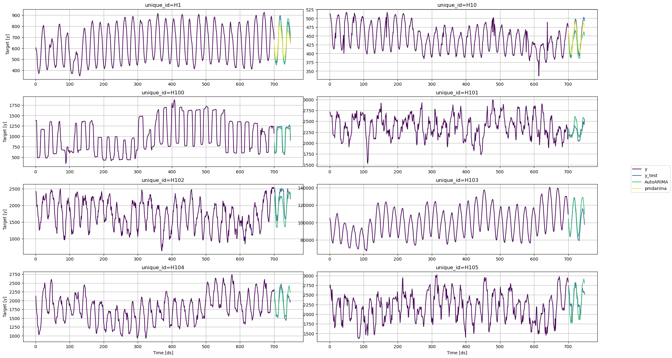
You can use the `StatsForecast` class to parallelize your own models. In
this section we will use it to run the `auto_arima` model from
`pmdarima`.
```python theme={null}
class PMDAutoARIMA(_TS):
def __init__(self, season_length: int):
self.season_length = season_length
def forecast(self, y, h, X=None, X_future=None, fitted=False):
mod = auto_arima_p(
y, m=self.season_length,
with_intercept=False #ensure comparability with Nixtla's implementation
)
return {'mean': mod.predict(h)}
def __repr__(self):
return 'pmdarima'
```
```python theme={null}
n_series_pmdarima = 2
```
```python theme={null}
fcst = StatsForecast(
df = train.query('unique_id in ["H1", "H10"]'),
models=[PMDAutoARIMA(season_length=24)],
freq='H',
n_jobs=-1
)
```
```python theme={null}
init = time.time()
forecast_pmdarima = fcst.forecast(48)
end = time.time()
time_pmdarima = end - init
time_pmdarima
```
```text theme={null}
886.2768685817719
```
```python theme={null}
forecast_pmdarima.head()
```
| | ds | pmdarima |
| ---------- | --- | ---------- |
| unique\_id | | |
| H1 | 701 | 628.310547 |
| H1 | 702 | 571.659851 |
| H1 | 703 | 543.504700 |
| H1 | 704 | 517.539062 |
| H1 | 705 | 502.829559 |
```python theme={null}
forecast_pmdarima = forecast_pmdarima.reset_index()
```
```python theme={null}
test = test.merge(forecast_pmdarima, how='left', on=['unique_id', 'ds'])
```
```python theme={null}
plot_series(train, test, plot_random=False)
```
## Alternatives
### pmdarima
You can use the `StatsForecast` class to parallelize your own models. In
this section we will use it to run the `auto_arima` model from
`pmdarima`.
```python theme={null}
class PMDAutoARIMA(_TS):
def __init__(self, season_length: int):
self.season_length = season_length
def forecast(self, y, h, X=None, X_future=None, fitted=False):
mod = auto_arima_p(
y, m=self.season_length,
with_intercept=False #ensure comparability with Nixtla's implementation
)
return {'mean': mod.predict(h)}
def __repr__(self):
return 'pmdarima'
```
```python theme={null}
n_series_pmdarima = 2
```
```python theme={null}
fcst = StatsForecast(
df = train.query('unique_id in ["H1", "H10"]'),
models=[PMDAutoARIMA(season_length=24)],
freq='H',
n_jobs=-1
)
```
```python theme={null}
init = time.time()
forecast_pmdarima = fcst.forecast(48)
end = time.time()
time_pmdarima = end - init
time_pmdarima
```
```text theme={null}
886.2768685817719
```
```python theme={null}
forecast_pmdarima.head()
```
| | ds | pmdarima |
| ---------- | --- | ---------- |
| unique\_id | | |
| H1 | 701 | 628.310547 |
| H1 | 702 | 571.659851 |
| H1 | 703 | 543.504700 |
| H1 | 704 | 517.539062 |
| H1 | 705 | 502.829559 |
```python theme={null}
forecast_pmdarima = forecast_pmdarima.reset_index()
```
```python theme={null}
test = test.merge(forecast_pmdarima, how='left', on=['unique_id', 'ds'])
```
```python theme={null}
plot_series(train, test, plot_random=False)
```
 ### Prophet
`Prophet` is designed to receive a pandas dataframe, so we cannot use
`StatForecast`. Therefore, we need to parallize from scratch.
```python theme={null}
params_grid = {'seasonality_mode': ['multiplicative','additive'],
'growth': ['linear', 'flat'],
'changepoint_prior_scale': [0.1, 0.2, 0.3, 0.4, 0.5],
'n_changepoints': [5, 10, 15, 20]}
grid = ParameterGrid(params_grid)
```
```python theme={null}
def fit_and_predict(index, ts):
df = ts.drop(columns='unique_id', axis=1)
max_ds = df['ds'].max()
df['ds'] = pd.date_range(start='1970-01-01', periods=df.shape[0], freq='H')
df_val = df.tail(48)
df_train = df.drop(df_val.index)
y_val = df_val['y'].values
if len(df_train) >= 48:
val_results = {'losses': [], 'params': []}
for params in grid:
model = Prophet(seasonality_mode=params['seasonality_mode'],
growth=params['growth'],
weekly_seasonality=True,
daily_seasonality=True,
yearly_seasonality=True,
n_changepoints=params['n_changepoints'],
changepoint_prior_scale=params['changepoint_prior_scale'])
model = model.fit(df_train)
forecast = model.make_future_dataframe(periods=48,
include_history=False,
freq='H')
forecast = model.predict(forecast)
forecast['unique_id'] = index
forecast = forecast.filter(items=['unique_id', 'ds', 'yhat'])
loss = np.mean(abs(y_val - forecast['yhat'].values))
val_results['losses'].append(loss)
val_results['params'].append(params)
idx_params = np.argmin(val_results['losses'])
params = val_results['params'][idx_params]
else:
params = {'seasonality_mode': 'multiplicative',
'growth': 'flat',
'n_changepoints': 150,
'changepoint_prior_scale': 0.5}
model = Prophet(seasonality_mode=params['seasonality_mode'],
growth=params['growth'],
weekly_seasonality=True,
daily_seasonality=True,
yearly_seasonality=True,
n_changepoints=params['n_changepoints'],
changepoint_prior_scale=params['changepoint_prior_scale'])
model = model.fit(df)
forecast = model.make_future_dataframe(periods=48,
include_history=False,
freq='H')
forecast = model.predict(forecast)
forecast.insert(0, 'unique_id', index)
forecast['ds'] = np.arange(max_ds + 1, max_ds + 48 + 1)
forecast = forecast.filter(items=['unique_id', 'ds', 'yhat'])
return forecast
```
```python theme={null}
init = time.time()
with Pool(cpu_count()) as pool:
forecast_prophet = pool.starmap(fit_and_predict, train.groupby('unique_id'))
end = time.time()
forecast_prophet = pd.concat(forecast_prophet).rename(columns={'yhat': 'prophet'})
time_prophet = end - init
time_prophet
```
```text theme={null}
120.7272641658783
```
```python theme={null}
forecast_prophet
```
| | unique\_id | ds | prophet |
| --- | ---------- | --- | ----------- |
| 0 | H1 | 701 | 635.914254 |
| 1 | H1 | 702 | 565.976464 |
| 2 | H1 | 703 | 505.095507 |
| 3 | H1 | 704 | 462.559539 |
| 4 | H1 | 705 | 438.766801 |
| ... | ... | ... | ... |
| 43 | H112 | 744 | 6184.686240 |
| 44 | H112 | 745 | 6188.851888 |
| 45 | H112 | 746 | 6129.306256 |
| 46 | H112 | 747 | 6058.040672 |
| 47 | H112 | 748 | 5991.982370 |
```python theme={null}
test = test.merge(forecast_prophet, how='left', on=['unique_id', 'ds'])
```
```python theme={null}
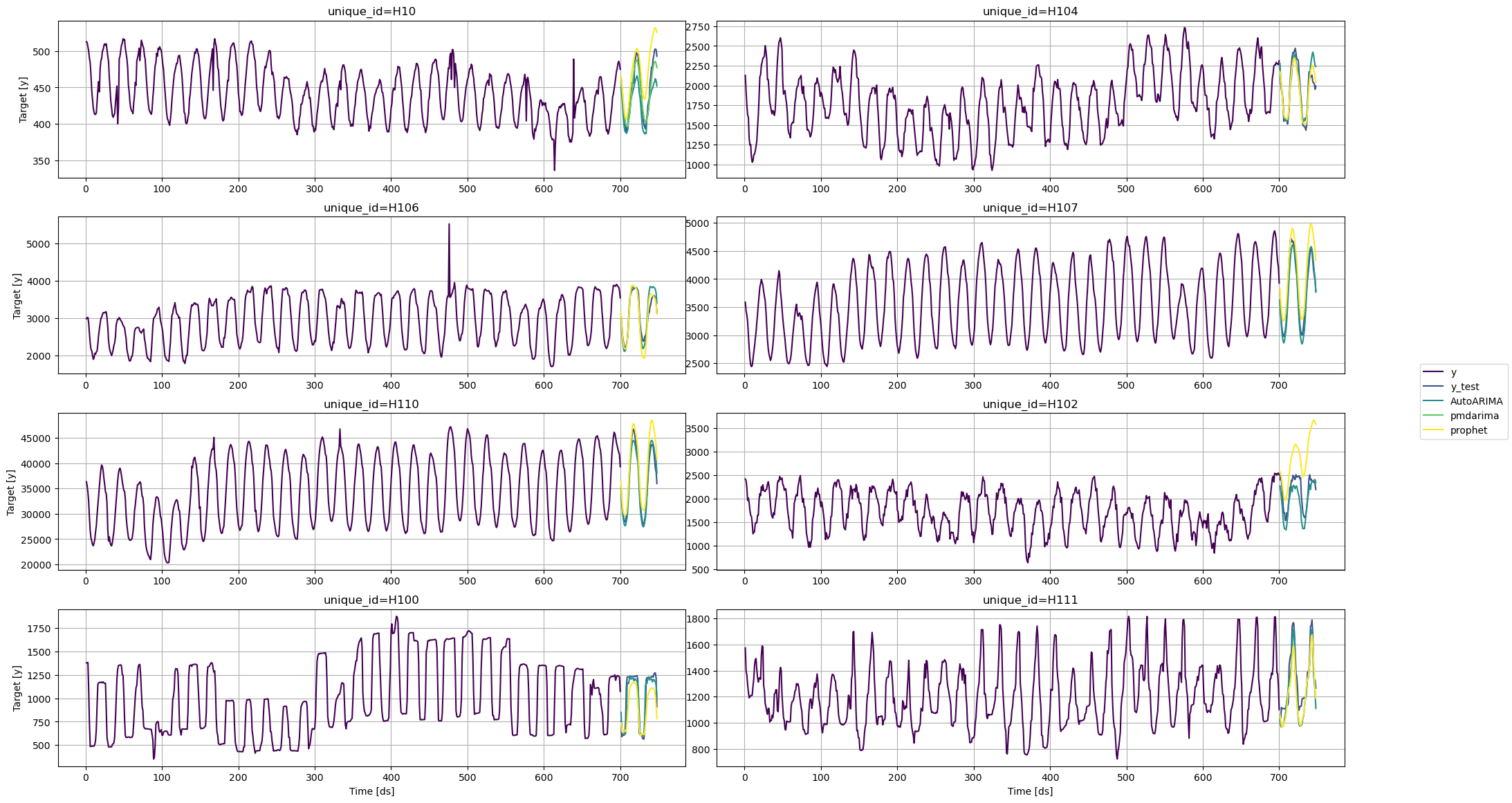
plot_series(train, test)
```
### Prophet
`Prophet` is designed to receive a pandas dataframe, so we cannot use
`StatForecast`. Therefore, we need to parallize from scratch.
```python theme={null}
params_grid = {'seasonality_mode': ['multiplicative','additive'],
'growth': ['linear', 'flat'],
'changepoint_prior_scale': [0.1, 0.2, 0.3, 0.4, 0.5],
'n_changepoints': [5, 10, 15, 20]}
grid = ParameterGrid(params_grid)
```
```python theme={null}
def fit_and_predict(index, ts):
df = ts.drop(columns='unique_id', axis=1)
max_ds = df['ds'].max()
df['ds'] = pd.date_range(start='1970-01-01', periods=df.shape[0], freq='H')
df_val = df.tail(48)
df_train = df.drop(df_val.index)
y_val = df_val['y'].values
if len(df_train) >= 48:
val_results = {'losses': [], 'params': []}
for params in grid:
model = Prophet(seasonality_mode=params['seasonality_mode'],
growth=params['growth'],
weekly_seasonality=True,
daily_seasonality=True,
yearly_seasonality=True,
n_changepoints=params['n_changepoints'],
changepoint_prior_scale=params['changepoint_prior_scale'])
model = model.fit(df_train)
forecast = model.make_future_dataframe(periods=48,
include_history=False,
freq='H')
forecast = model.predict(forecast)
forecast['unique_id'] = index
forecast = forecast.filter(items=['unique_id', 'ds', 'yhat'])
loss = np.mean(abs(y_val - forecast['yhat'].values))
val_results['losses'].append(loss)
val_results['params'].append(params)
idx_params = np.argmin(val_results['losses'])
params = val_results['params'][idx_params]
else:
params = {'seasonality_mode': 'multiplicative',
'growth': 'flat',
'n_changepoints': 150,
'changepoint_prior_scale': 0.5}
model = Prophet(seasonality_mode=params['seasonality_mode'],
growth=params['growth'],
weekly_seasonality=True,
daily_seasonality=True,
yearly_seasonality=True,
n_changepoints=params['n_changepoints'],
changepoint_prior_scale=params['changepoint_prior_scale'])
model = model.fit(df)
forecast = model.make_future_dataframe(periods=48,
include_history=False,
freq='H')
forecast = model.predict(forecast)
forecast.insert(0, 'unique_id', index)
forecast['ds'] = np.arange(max_ds + 1, max_ds + 48 + 1)
forecast = forecast.filter(items=['unique_id', 'ds', 'yhat'])
return forecast
```
```python theme={null}
init = time.time()
with Pool(cpu_count()) as pool:
forecast_prophet = pool.starmap(fit_and_predict, train.groupby('unique_id'))
end = time.time()
forecast_prophet = pd.concat(forecast_prophet).rename(columns={'yhat': 'prophet'})
time_prophet = end - init
time_prophet
```
```text theme={null}
120.7272641658783
```
```python theme={null}
forecast_prophet
```
| | unique\_id | ds | prophet |
| --- | ---------- | --- | ----------- |
| 0 | H1 | 701 | 635.914254 |
| 1 | H1 | 702 | 565.976464 |
| 2 | H1 | 703 | 505.095507 |
| 3 | H1 | 704 | 462.559539 |
| 4 | H1 | 705 | 438.766801 |
| ... | ... | ... | ... |
| 43 | H112 | 744 | 6184.686240 |
| 44 | H112 | 745 | 6188.851888 |
| 45 | H112 | 746 | 6129.306256 |
| 46 | H112 | 747 | 6058.040672 |
| 47 | H112 | 748 | 5991.982370 |
```python theme={null}
test = test.merge(forecast_prophet, how='left', on=['unique_id', 'ds'])
```
```python theme={null}
plot_series(train, test)
```
 ### Evaluation
### Time
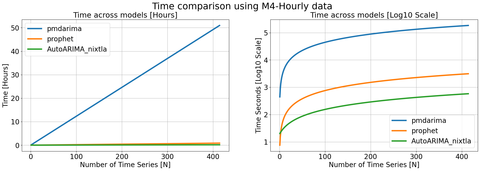
Since `AutoARIMA` works with numba is useful to calculate the time for
just one time series.
```python theme={null}
fcst = StatsForecast(df=train.query('unique_id == "H1"'),
models=models, freq='H',
n_jobs=1)
```
```python theme={null}
init = time.time()
forecasts = fcst.forecast(48)
end = time.time()
time_nixtla_1 = end - init
time_nixtla_1
```
```text theme={null}
18.752424716949463
```
```python theme={null}
times = pd.DataFrame({'n_series': np.arange(1, 414 + 1)})
times['pmdarima'] = time_pmdarima * times['n_series'] / n_series_pmdarima
times['prophet'] = time_prophet * times['n_series'] / n_series
times['AutoARIMA_nixtla'] = time_nixtla_1 + times['n_series'] * (time_nixtla - time_nixtla_1) / n_series
times = times.set_index('n_series')
```
```python theme={null}
times.tail(5)
```
| | pmdarima | prophet | AutoARIMA\_nixtla |
| --------- | ------------- | ----------- | ----------------- |
| n\_series | | | |
| 410 | 181686.758059 | 3093.636144 | 573.128222 |
| 411 | 182129.896494 | 3101.181598 | 574.480358 |
| 412 | 182573.034928 | 3108.727052 | 575.832494 |
| 413 | 183016.173362 | 3116.272506 | 577.184630 |
| 414 | 183459.311796 | 3123.817960 | 578.536766 |
```python theme={null}
fig, axes = plt.subplots(1, 2, figsize = (24, 7))
(times/3600).plot(ax=axes[0], linewidth=4)
np.log10(times).plot(ax=axes[1], linewidth=4)
axes[0].set_title('Time across models [Hours]', fontsize=22)
axes[1].set_title('Time across models [Log10 Scale]', fontsize=22)
axes[0].set_ylabel('Time [Hours]', fontsize=20)
axes[1].set_ylabel('Time Seconds [Log10 Scale]', fontsize=20)
fig.suptitle('Time comparison using M4-Hourly data', fontsize=27)
for ax in axes:
ax.set_xlabel('Number of Time Series [N]', fontsize=20)
ax.legend(prop={'size': 20})
ax.grid()
for label in (ax.get_xticklabels() + ax.get_yticklabels()):
label.set_fontsize(20)
```
### Evaluation
### Time
Since `AutoARIMA` works with numba is useful to calculate the time for
just one time series.
```python theme={null}
fcst = StatsForecast(df=train.query('unique_id == "H1"'),
models=models, freq='H',
n_jobs=1)
```
```python theme={null}
init = time.time()
forecasts = fcst.forecast(48)
end = time.time()
time_nixtla_1 = end - init
time_nixtla_1
```
```text theme={null}
18.752424716949463
```
```python theme={null}
times = pd.DataFrame({'n_series': np.arange(1, 414 + 1)})
times['pmdarima'] = time_pmdarima * times['n_series'] / n_series_pmdarima
times['prophet'] = time_prophet * times['n_series'] / n_series
times['AutoARIMA_nixtla'] = time_nixtla_1 + times['n_series'] * (time_nixtla - time_nixtla_1) / n_series
times = times.set_index('n_series')
```
```python theme={null}
times.tail(5)
```
| | pmdarima | prophet | AutoARIMA\_nixtla |
| --------- | ------------- | ----------- | ----------------- |
| n\_series | | | |
| 410 | 181686.758059 | 3093.636144 | 573.128222 |
| 411 | 182129.896494 | 3101.181598 | 574.480358 |
| 412 | 182573.034928 | 3108.727052 | 575.832494 |
| 413 | 183016.173362 | 3116.272506 | 577.184630 |
| 414 | 183459.311796 | 3123.817960 | 578.536766 |
```python theme={null}
fig, axes = plt.subplots(1, 2, figsize = (24, 7))
(times/3600).plot(ax=axes[0], linewidth=4)
np.log10(times).plot(ax=axes[1], linewidth=4)
axes[0].set_title('Time across models [Hours]', fontsize=22)
axes[1].set_title('Time across models [Log10 Scale]', fontsize=22)
axes[0].set_ylabel('Time [Hours]', fontsize=20)
axes[1].set_ylabel('Time Seconds [Log10 Scale]', fontsize=20)
fig.suptitle('Time comparison using M4-Hourly data', fontsize=27)
for ax in axes:
ax.set_xlabel('Number of Time Series [N]', fontsize=20)
ax.legend(prop={'size': 20})
ax.grid()
for label in (ax.get_xticklabels() + ax.get_yticklabels()):
label.set_fontsize(20)
```
 ```python theme={null}
fig.savefig('computational-efficiency.png', dpi=300)
```
### Performance
#### pmdarima (only two time series)
```python theme={null}
name_models = test.drop(columns=['unique_id', 'ds', 'y_test']).columns.tolist()
```
```python theme={null}
test_pmdarima = test.query('unique_id in ["H1", "H10"]')
eval_pmdarima = []
for model in name_models:
mae = np.mean(abs(test_pmdarima[model] - test_pmdarima['y_test']))
eval_pmdarima.append({'model': model, 'mae': mae})
pd.DataFrame(eval_pmdarima).sort_values('mae')
```
| | model | mae |
| - | --------- | --------- |
| 0 | AutoARIMA | 20.289669 |
| 1 | pmdarima | 24.676279 |
| 2 | prophet | 39.201933 |
#### Prophet
```python theme={null}
eval_prophet = []
for model in name_models:
if 'pmdarima' in model:
continue
mae = np.mean(abs(test[model] - test['y_test']))
eval_prophet.append({'model': model, 'mae': mae})
pd.DataFrame(eval_prophet).sort_values('mae')
```
| | model | mae |
| - | --------- | ----------- |
| 0 | AutoARIMA | 680.202965 |
| 1 | prophet | 1058.578963 |
For a complete comparison check the [complete
experiment](https://github.com/Nixtla/statsforecast/tree/v0.6.0/experiments/arima).
```python theme={null}
fig.savefig('computational-efficiency.png', dpi=300)
```
### Performance
#### pmdarima (only two time series)
```python theme={null}
name_models = test.drop(columns=['unique_id', 'ds', 'y_test']).columns.tolist()
```
```python theme={null}
test_pmdarima = test.query('unique_id in ["H1", "H10"]')
eval_pmdarima = []
for model in name_models:
mae = np.mean(abs(test_pmdarima[model] - test_pmdarima['y_test']))
eval_pmdarima.append({'model': model, 'mae': mae})
pd.DataFrame(eval_pmdarima).sort_values('mae')
```
| | model | mae |
| - | --------- | --------- |
| 0 | AutoARIMA | 20.289669 |
| 1 | pmdarima | 24.676279 |
| 2 | prophet | 39.201933 |
#### Prophet
```python theme={null}
eval_prophet = []
for model in name_models:
if 'pmdarima' in model:
continue
mae = np.mean(abs(test[model] - test['y_test']))
eval_prophet.append({'model': model, 'mae': mae})
pd.DataFrame(eval_prophet).sort_values('mae')
```
| | model | mae |
| - | --------- | ----------- |
| 0 | AutoARIMA | 680.202965 |
| 1 | prophet | 1058.578963 |
For a complete comparison check the [complete
experiment](https://github.com/Nixtla/statsforecast/tree/v0.6.0/experiments/arima).