> ## Documentation Index
> Fetch the complete documentation index at: https://nixtlaverse.nixtla.io/llms.txt
> Use this file to discover all available pages before exploring further.
# Probabilistic Forecasting | NeuralForecast
> Quantify uncertainty
Probabilistic forecasting is a natural answer to quantify the
uncertainty of target variable’s future. The task requires to model the
following conditional predictive distribution:
$\mathbb{P}(\mathbf{y}_{t+1:t+H} \;|\; \mathbf{y}_{:t})$
We will show you how to tackle the task with `NeuralForecast` by
combining a classic Long Short Term Memory Network
[(LSTM)](https://arxiv.org/abs/2201.12886) and the Neural Hierarchical
Interpolation [(NHITS)](https://arxiv.org/abs/2201.12886) with the multi
quantile loss function (MQLoss).
$\mathrm{MQLoss}(y_{\tau}, [\hat{y}^{(q1)}_{\tau},\hat{y}^{(q2)}_{\tau},\dots,\hat{y}^{(Q)}_{\tau}]) = \frac{1}{H} \sum_{q} \mathrm{QL}(y_{\tau}, \hat{y}^{(q)}_{\tau})$
In this notebook we will:
1. Install NeuralForecast Library
2.
Explore the M4-Hourly data.
3. Train the LSTM and NHITS
4.
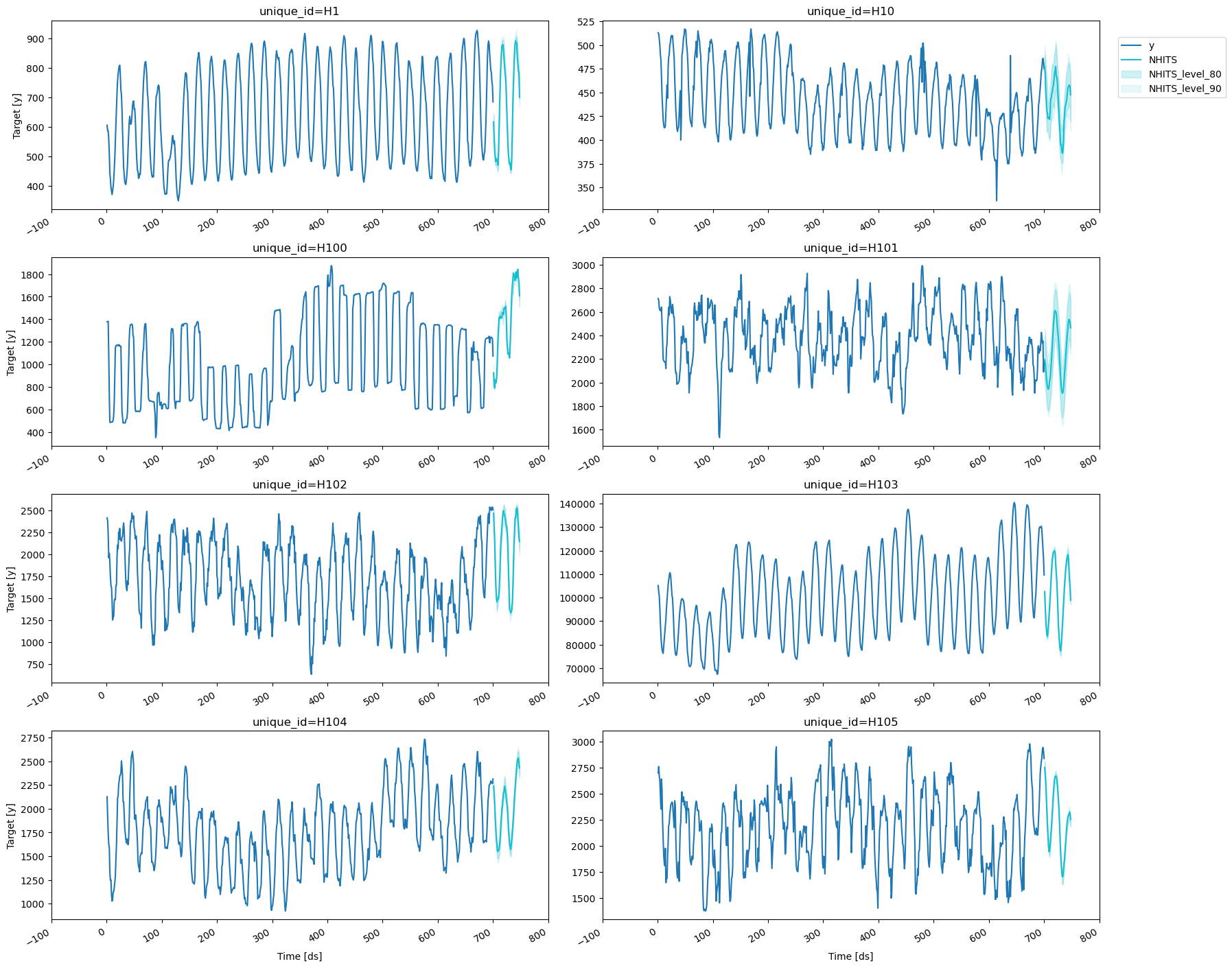
Visualize the LSTM/NHITS prediction intervals.
You can run these experiments using GPU with Google Colab.
 ## 1. Installing NeuralForecast
```python theme={null}
%%capture
!pip install neuralforecast
```
#### Useful functions
The `plot_grid` auxiliary function defined below will be useful to plot
different time series, and different models’ forecasts.
```python theme={null}
import logging
import warnings
import torch
from utilsforecast.plotting import plot_series
```
```python theme={null}
warnings.filterwarnings("ignore")
```
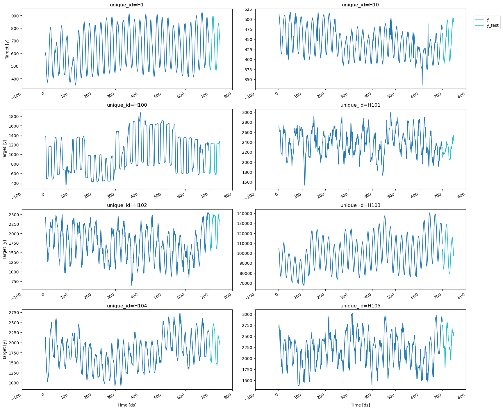
## 2. Loading M4 Data
For testing purposes, we will use the Hourly dataset from the [M4
competition](https://www.researchgate.net/publication/325901666_The_M4_Competition_Results_findings_conclusion_and_way_forward).
```python theme={null}
import pandas as pd
```
```python theme={null}
Y_train_df = pd.read_csv('https://auto-arima-results.s3.amazonaws.com/M4-Hourly.csv')
Y_test_df = pd.read_csv(
'https://auto-arima-results.s3.amazonaws.com/M4-Hourly-test.csv'
).rename(columns={'y': 'y_test'})
```
In this example we will use a subset of the data to avoid waiting too
long. You can modify the number of series if you want.
```python theme={null}
n_series = 8
uids = Y_train_df['unique_id'].unique()[:n_series]
Y_train_df = Y_train_df.query('unique_id in @uids')
Y_test_df = Y_test_df.query('unique_id in @uids')
```
```python theme={null}
plot_series(Y_train_df, Y_test_df)
```
## 1. Installing NeuralForecast
```python theme={null}
%%capture
!pip install neuralforecast
```
#### Useful functions
The `plot_grid` auxiliary function defined below will be useful to plot
different time series, and different models’ forecasts.
```python theme={null}
import logging
import warnings
import torch
from utilsforecast.plotting import plot_series
```
```python theme={null}
warnings.filterwarnings("ignore")
```
## 2. Loading M4 Data
For testing purposes, we will use the Hourly dataset from the [M4
competition](https://www.researchgate.net/publication/325901666_The_M4_Competition_Results_findings_conclusion_and_way_forward).
```python theme={null}
import pandas as pd
```
```python theme={null}
Y_train_df = pd.read_csv('https://auto-arima-results.s3.amazonaws.com/M4-Hourly.csv')
Y_test_df = pd.read_csv(
'https://auto-arima-results.s3.amazonaws.com/M4-Hourly-test.csv'
).rename(columns={'y': 'y_test'})
```
In this example we will use a subset of the data to avoid waiting too
long. You can modify the number of series if you want.
```python theme={null}
n_series = 8
uids = Y_train_df['unique_id'].unique()[:n_series]
Y_train_df = Y_train_df.query('unique_id in @uids')
Y_test_df = Y_test_df.query('unique_id in @uids')
```
```python theme={null}
plot_series(Y_train_df, Y_test_df)
```
 ## 3. Model Training
The `core.NeuralForecast` provides a high-level interface with our
collection of PyTorch models. `NeuralForecast` is instantiated with a
list of `models=[LSTM(...), NHITS(...)]`, configured for the forecasting
task.
* The `horizon` parameter controls the number of steps ahead of the
predictions, in this example 48 hours ahead (2 days).
* The `MQLoss` with `levels=[80,90]` specializes the network’s output
into the 80% and 90% prediction intervals.
* The `max_steps=2000`, controls the duration of the network’s
training.
For more network’s instantiation details check their
[documentation](https://nixtlaverse.nixtla.io/neuralforecast/models.dilated_rnn.html).
```python theme={null}
from neuralforecast import NeuralForecast
from neuralforecast.losses.pytorch import MQLoss
from neuralforecast.models import LSTM, NHITS
```
```python theme={null}
logging.getLogger('pytorch_lightning').setLevel(logging.ERROR)
torch.set_float32_matmul_precision('high')
```
```python theme={null}
horizon = 48
levels = [80, 90]
models = [LSTM(input_size=3*horizon, h=horizon,
loss=MQLoss(level=levels), max_steps=1000),
NHITS(input_size=7*horizon, h=horizon,
n_freq_downsample=[24, 12, 1],
loss=MQLoss(level=levels), max_steps=2000),]
nf = NeuralForecast(models=models, freq=1)
```
```text theme={null}
Seed set to 1
Seed set to 1
```
All the models of the library are global, meaning that all time series
in `Y_train_df` is used during a shared optimization to train a single
model with shared parameters. This is the most common practice in the
forecasting literature for deep learning models, and it is known as
“cross-learning”.
```python theme={null}
%%capture
nf.fit(df=Y_train_df)
```
```python theme={null}
Y_hat_df = nf.predict()
Y_hat_df.head()
```
```text theme={null}
Predicting: | | 0/? [00:00
### NHITS
```python theme={null}
plot_series(Y_train_df, Y_test_df, level=levels, models=['NHITS'])
```
## 3. Model Training
The `core.NeuralForecast` provides a high-level interface with our
collection of PyTorch models. `NeuralForecast` is instantiated with a
list of `models=[LSTM(...), NHITS(...)]`, configured for the forecasting
task.
* The `horizon` parameter controls the number of steps ahead of the
predictions, in this example 48 hours ahead (2 days).
* The `MQLoss` with `levels=[80,90]` specializes the network’s output
into the 80% and 90% prediction intervals.
* The `max_steps=2000`, controls the duration of the network’s
training.
For more network’s instantiation details check their
[documentation](https://nixtlaverse.nixtla.io/neuralforecast/models.dilated_rnn.html).
```python theme={null}
from neuralforecast import NeuralForecast
from neuralforecast.losses.pytorch import MQLoss
from neuralforecast.models import LSTM, NHITS
```
```python theme={null}
logging.getLogger('pytorch_lightning').setLevel(logging.ERROR)
torch.set_float32_matmul_precision('high')
```
```python theme={null}
horizon = 48
levels = [80, 90]
models = [LSTM(input_size=3*horizon, h=horizon,
loss=MQLoss(level=levels), max_steps=1000),
NHITS(input_size=7*horizon, h=horizon,
n_freq_downsample=[24, 12, 1],
loss=MQLoss(level=levels), max_steps=2000),]
nf = NeuralForecast(models=models, freq=1)
```
```text theme={null}
Seed set to 1
Seed set to 1
```
All the models of the library are global, meaning that all time series
in `Y_train_df` is used during a shared optimization to train a single
model with shared parameters. This is the most common practice in the
forecasting literature for deep learning models, and it is known as
“cross-learning”.
```python theme={null}
%%capture
nf.fit(df=Y_train_df)
```
```python theme={null}
Y_hat_df = nf.predict()
Y_hat_df.head()
```
```text theme={null}
Predicting: | | 0/? [00:00
### NHITS
```python theme={null}
plot_series(Y_train_df, Y_test_df, level=levels, models=['NHITS'])
```
 ## References
* [Roger Koenker and Gilbert Basset (1978). Regression Quantiles,
Econometrica.](https://www.jstor.org/stable/1913643)
## References
* [Roger Koenker and Gilbert Basset (1978). Regression Quantiles,
Econometrica.](https://www.jstor.org/stable/1913643)
* [Jeffrey L. Elman (1990). “Finding Structure in
Time”.](https://onlinelibrary.wiley.com/doi/abs/10.1207/s15516709cog1402_1)
* [Cristian Challu, Kin G. Olivares, Boris N. Oreshkin, Federico
Garza, Max Mergenthaler-Canseco, Artur Dubrawski (2021). NHITS:
Neural Hierarchical Interpolation for Time Series Forecasting.
Accepted at AAAI 2023.](https://arxiv.org/abs/2201.12886)