> ## Documentation Index
> Fetch the complete documentation index at: https://nixtlaverse.nixtla.io/llms.txt
> Use this file to discover all available pages before exploring further.
# Long-Horizon Forecasting with Transformer models
> Tutorial on how to train and forecast Transformer models.
Transformer models, originally proposed for applications in natural
language processing, have seen increasing adoption in the field of time
series forecasting. The transformative power of these models lies in
their novel architecture that relies heavily on the self-attention
mechanism, which helps the model to focus on different parts of the
input sequence to make predictions, while capturing long-range
dependencies within the data. In the context of time series forecasting,
Transformer models leverage this self-attention mechanism to identify
relevant information across different periods in the time series, making
them exceptionally effective in predicting future values for complex and
noisy sequences.
Long horizon forecasting consists of predicting a large number of
timestamps. It is a challenging task because of the *volatility* of the
predictions and the *computational complexity*. To solve this problem,
recent studies proposed a variety of Transformer-based models.
The Neuralforecast library includes implementations of the following
popular recent models: `Informer` (Zhou, H. et al. 2021), `Autoformer`
(Wu et al. 2021), `FEDformer` (Zhou, T. et al. 2022), and `PatchTST`
(Nie et al. 2023).
Our implementation of all these models are univariate, meaning that only
autoregressive values of each feature are used for forecasting. **We
observed that these unvivariate models are more accurate and faster than
their multivariate couterpart**.
In this notebook we will show how to: \* Load the
[ETTm2](https://github.com/zhouhaoyi/ETDataset) benchmark dataset, used
in the academic literature. \* Train models \* Forecast the test set
**The results achieved in this notebook outperform the original
self-reported results in the respective original paper, with a fraction
of the computational cost. Additionally, all models are trained with the
default recommended parameters, results can be further improved using
our `auto` models with automatic hyperparameter selection.**
You can run these experiments using GPU with Google Colab.
 ## 1. Installing libraries
```python theme={null}
%%capture
!pip install neuralforecast datasetsforecast utilsforecast
```
## 2. Load ETTm2 Data
The `LongHorizon` class will automatically download the complete ETTm2
dataset and process it.
It return three Dataframes: `Y_df` contains the values for the target
variables, `X_df` contains exogenous calendar features and `S_df`
contains static features for each time-series (none for ETTm2). For this
example we will only use `Y_df`.
If you want to use your own data just replace `Y_df`. Be sure to use a
long format and have a similar structure to our data set.
```python theme={null}
import pandas as pd
from datasetsforecast.long_horizon import LongHorizon
```
```python theme={null}
# Change this to your own data to try the model
Y_df, _, _ = LongHorizon.load(directory='./', group='ETTm2')
Y_df['ds'] = pd.to_datetime(Y_df['ds'])
n_time = len(Y_df.ds.unique())
val_size = int(.2 * n_time)
test_size = int(.2 * n_time)
Y_df.groupby('unique_id').head(2)
```
| | unique\_id | ds | y |
| ------ | ---------- | ------------------- | --------- |
| 0 | HUFL | 2016-07-01 00:00:00 | -0.041413 |
| 1 | HUFL | 2016-07-01 00:15:00 | -0.185467 |
| 57600 | HULL | 2016-07-01 00:00:00 | 0.040104 |
| 57601 | HULL | 2016-07-01 00:15:00 | -0.214450 |
| 115200 | LUFL | 2016-07-01 00:00:00 | 0.695804 |
| 115201 | LUFL | 2016-07-01 00:15:00 | 0.434685 |
| 172800 | LULL | 2016-07-01 00:00:00 | 0.434430 |
| 172801 | LULL | 2016-07-01 00:15:00 | 0.428168 |
| 230400 | MUFL | 2016-07-01 00:00:00 | -0.599211 |
| 230401 | MUFL | 2016-07-01 00:15:00 | -0.658068 |
| 288000 | MULL | 2016-07-01 00:00:00 | -0.393536 |
| 288001 | MULL | 2016-07-01 00:15:00 | -0.659338 |
| 345600 | OT | 2016-07-01 00:00:00 | 1.018032 |
| 345601 | OT | 2016-07-01 00:15:00 | 0.980124 |
## 3. Train models
We will train models using the `cross_validation` method, which allows
users to automatically simulate multiple historic forecasts (in the test
set).
The `cross_validation` method will use the validation set for
hyperparameter selection and early stopping, and will then produce the
forecasts for the test set.
First, instantiate each model in the `models` list, specifying the
`horizon`, `input_size`, and training iterations.
(NOTE: The `FEDformer` model was excluded due to extremely long training
times.)
```python theme={null}
%%capture
from neuralforecast.core import NeuralForecast
from neuralforecast.models import Informer, Autoformer, FEDformer, PatchTST
```
```text theme={null}
INFO:torch.distributed.nn.jit.instantiator:Created a temporary directory at /tmp/tmpopb2vyyt
INFO:torch.distributed.nn.jit.instantiator:Writing /tmp/tmpopb2vyyt/_remote_module_non_scriptable.py
```
```python theme={null}
%%capture
horizon = 96 # 24hrs = 4 * 15 min.
models = [Informer(h=horizon, # Forecasting horizon
input_size=horizon, # Input size
max_steps=1000, # Number of training iterations
val_check_steps=100, # Compute validation loss every 100 steps
early_stop_patience_steps=3), # Stop training if validation loss does not improve
Autoformer(h=horizon,
input_size=horizon,
max_steps=1000,
val_check_steps=100,
early_stop_patience_steps=3),
PatchTST(h=horizon,
input_size=horizon,
max_steps=1000,
val_check_steps=100,
early_stop_patience_steps=3),
]
```
```text theme={null}
INFO:lightning_fabric.utilities.seed:Global seed set to 1
INFO:lightning_fabric.utilities.seed:Global seed set to 1
INFO:lightning_fabric.utilities.seed:Global seed set to 1
```
> **Tip**
>
> Check our `auto` models for automatic hyperparameter optimization.
Instantiate a `NeuralForecast` object with the following required
parameters:
* `models`: a list of models.
* `freq`: a string indicating the frequency of the data. (See [panda’s
available
frequencies](https://pandas.pydata.org/pandas-docs/stable/user_guide/timeseries.html#offset-aliases).)
Second, use the `cross_validation` method, specifying the dataset
(`Y_df`), validation size and test size.
```python theme={null}
%%capture
nf = NeuralForecast(
models=models,
freq='15min')
Y_hat_df = nf.cross_validation(df=Y_df,
val_size=val_size,
test_size=test_size,
n_windows=None)
```
The `cross_validation` method will return the forecasts for each model
on the test set.
```python theme={null}
Y_hat_df.head()
```
| | unique\_id | ds | cutoff | Informer | Autoformer | PatchTST | y |
| - | ---------- | ------------------- | ------------------- | --------- | ---------- | --------- | --------- |
| 0 | HUFL | 2017-10-24 00:00:00 | 2017-10-23 23:45:00 | -1.055062 | -0.861487 | -0.860189 | -0.977673 |
| 1 | HUFL | 2017-10-24 00:15:00 | 2017-10-23 23:45:00 | -1.021247 | -0.873399 | -0.865730 | -0.865620 |
| 2 | HUFL | 2017-10-24 00:30:00 | 2017-10-23 23:45:00 | -1.057297 | -0.900345 | -0.944296 | -0.961624 |
| 3 | HUFL | 2017-10-24 00:45:00 | 2017-10-23 23:45:00 | -0.886652 | -0.867466 | -0.974849 | -1.049700 |
| 4 | HUFL | 2017-10-24 01:00:00 | 2017-10-23 23:45:00 | -1.000431 | -0.887454 | -1.008530 | -0.953600 |
## 4. Evaluate Results
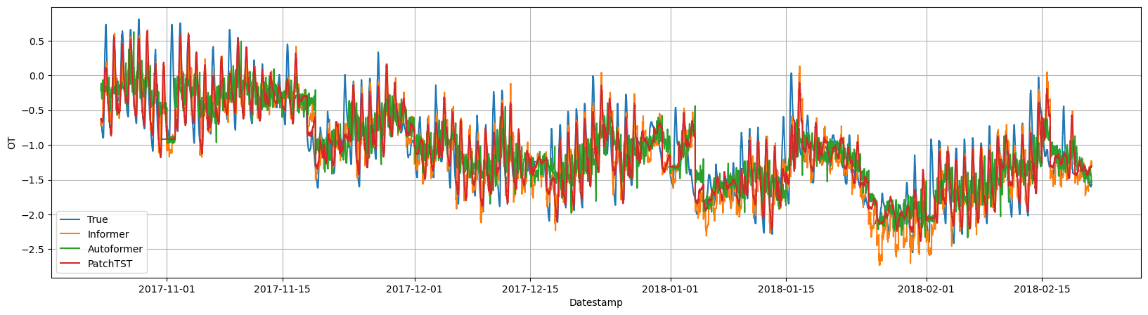
Next, we plot the forecasts on the test set for the `OT` variable for
all models.
```python theme={null}
import matplotlib.pyplot as plt
```
```python theme={null}
Y_plot = Y_hat_df[Y_hat_df['unique_id']=='OT'] # OT dataset
cutoffs = Y_hat_df['cutoff'].unique()[::horizon]
Y_plot = Y_plot[Y_hat_df['cutoff'].isin(cutoffs)]
plt.figure(figsize=(20,5))
plt.plot(Y_plot['ds'], Y_plot['y'], label='True')
plt.plot(Y_plot['ds'], Y_plot['Informer'], label='Informer')
plt.plot(Y_plot['ds'], Y_plot['Autoformer'], label='Autoformer')
plt.plot(Y_plot['ds'], Y_plot['PatchTST'], label='PatchTST')
plt.xlabel('Datestamp')
plt.ylabel('OT')
plt.grid()
plt.legend()
```
## 1. Installing libraries
```python theme={null}
%%capture
!pip install neuralforecast datasetsforecast utilsforecast
```
## 2. Load ETTm2 Data
The `LongHorizon` class will automatically download the complete ETTm2
dataset and process it.
It return three Dataframes: `Y_df` contains the values for the target
variables, `X_df` contains exogenous calendar features and `S_df`
contains static features for each time-series (none for ETTm2). For this
example we will only use `Y_df`.
If you want to use your own data just replace `Y_df`. Be sure to use a
long format and have a similar structure to our data set.
```python theme={null}
import pandas as pd
from datasetsforecast.long_horizon import LongHorizon
```
```python theme={null}
# Change this to your own data to try the model
Y_df, _, _ = LongHorizon.load(directory='./', group='ETTm2')
Y_df['ds'] = pd.to_datetime(Y_df['ds'])
n_time = len(Y_df.ds.unique())
val_size = int(.2 * n_time)
test_size = int(.2 * n_time)
Y_df.groupby('unique_id').head(2)
```
| | unique\_id | ds | y |
| ------ | ---------- | ------------------- | --------- |
| 0 | HUFL | 2016-07-01 00:00:00 | -0.041413 |
| 1 | HUFL | 2016-07-01 00:15:00 | -0.185467 |
| 57600 | HULL | 2016-07-01 00:00:00 | 0.040104 |
| 57601 | HULL | 2016-07-01 00:15:00 | -0.214450 |
| 115200 | LUFL | 2016-07-01 00:00:00 | 0.695804 |
| 115201 | LUFL | 2016-07-01 00:15:00 | 0.434685 |
| 172800 | LULL | 2016-07-01 00:00:00 | 0.434430 |
| 172801 | LULL | 2016-07-01 00:15:00 | 0.428168 |
| 230400 | MUFL | 2016-07-01 00:00:00 | -0.599211 |
| 230401 | MUFL | 2016-07-01 00:15:00 | -0.658068 |
| 288000 | MULL | 2016-07-01 00:00:00 | -0.393536 |
| 288001 | MULL | 2016-07-01 00:15:00 | -0.659338 |
| 345600 | OT | 2016-07-01 00:00:00 | 1.018032 |
| 345601 | OT | 2016-07-01 00:15:00 | 0.980124 |
## 3. Train models
We will train models using the `cross_validation` method, which allows
users to automatically simulate multiple historic forecasts (in the test
set).
The `cross_validation` method will use the validation set for
hyperparameter selection and early stopping, and will then produce the
forecasts for the test set.
First, instantiate each model in the `models` list, specifying the
`horizon`, `input_size`, and training iterations.
(NOTE: The `FEDformer` model was excluded due to extremely long training
times.)
```python theme={null}
%%capture
from neuralforecast.core import NeuralForecast
from neuralforecast.models import Informer, Autoformer, FEDformer, PatchTST
```
```text theme={null}
INFO:torch.distributed.nn.jit.instantiator:Created a temporary directory at /tmp/tmpopb2vyyt
INFO:torch.distributed.nn.jit.instantiator:Writing /tmp/tmpopb2vyyt/_remote_module_non_scriptable.py
```
```python theme={null}
%%capture
horizon = 96 # 24hrs = 4 * 15 min.
models = [Informer(h=horizon, # Forecasting horizon
input_size=horizon, # Input size
max_steps=1000, # Number of training iterations
val_check_steps=100, # Compute validation loss every 100 steps
early_stop_patience_steps=3), # Stop training if validation loss does not improve
Autoformer(h=horizon,
input_size=horizon,
max_steps=1000,
val_check_steps=100,
early_stop_patience_steps=3),
PatchTST(h=horizon,
input_size=horizon,
max_steps=1000,
val_check_steps=100,
early_stop_patience_steps=3),
]
```
```text theme={null}
INFO:lightning_fabric.utilities.seed:Global seed set to 1
INFO:lightning_fabric.utilities.seed:Global seed set to 1
INFO:lightning_fabric.utilities.seed:Global seed set to 1
```
> **Tip**
>
> Check our `auto` models for automatic hyperparameter optimization.
Instantiate a `NeuralForecast` object with the following required
parameters:
* `models`: a list of models.
* `freq`: a string indicating the frequency of the data. (See [panda’s
available
frequencies](https://pandas.pydata.org/pandas-docs/stable/user_guide/timeseries.html#offset-aliases).)
Second, use the `cross_validation` method, specifying the dataset
(`Y_df`), validation size and test size.
```python theme={null}
%%capture
nf = NeuralForecast(
models=models,
freq='15min')
Y_hat_df = nf.cross_validation(df=Y_df,
val_size=val_size,
test_size=test_size,
n_windows=None)
```
The `cross_validation` method will return the forecasts for each model
on the test set.
```python theme={null}
Y_hat_df.head()
```
| | unique\_id | ds | cutoff | Informer | Autoformer | PatchTST | y |
| - | ---------- | ------------------- | ------------------- | --------- | ---------- | --------- | --------- |
| 0 | HUFL | 2017-10-24 00:00:00 | 2017-10-23 23:45:00 | -1.055062 | -0.861487 | -0.860189 | -0.977673 |
| 1 | HUFL | 2017-10-24 00:15:00 | 2017-10-23 23:45:00 | -1.021247 | -0.873399 | -0.865730 | -0.865620 |
| 2 | HUFL | 2017-10-24 00:30:00 | 2017-10-23 23:45:00 | -1.057297 | -0.900345 | -0.944296 | -0.961624 |
| 3 | HUFL | 2017-10-24 00:45:00 | 2017-10-23 23:45:00 | -0.886652 | -0.867466 | -0.974849 | -1.049700 |
| 4 | HUFL | 2017-10-24 01:00:00 | 2017-10-23 23:45:00 | -1.000431 | -0.887454 | -1.008530 | -0.953600 |
## 4. Evaluate Results
Next, we plot the forecasts on the test set for the `OT` variable for
all models.
```python theme={null}
import matplotlib.pyplot as plt
```
```python theme={null}
Y_plot = Y_hat_df[Y_hat_df['unique_id']=='OT'] # OT dataset
cutoffs = Y_hat_df['cutoff'].unique()[::horizon]
Y_plot = Y_plot[Y_hat_df['cutoff'].isin(cutoffs)]
plt.figure(figsize=(20,5))
plt.plot(Y_plot['ds'], Y_plot['y'], label='True')
plt.plot(Y_plot['ds'], Y_plot['Informer'], label='Informer')
plt.plot(Y_plot['ds'], Y_plot['Autoformer'], label='Autoformer')
plt.plot(Y_plot['ds'], Y_plot['PatchTST'], label='PatchTST')
plt.xlabel('Datestamp')
plt.ylabel('OT')
plt.grid()
plt.legend()
```
 Finally, we compute the test errors using the Mean Absolute Error (MAE):
$\qquad MAE = \frac{1}{Windows * Horizon} \sum_{\tau} |y_{\tau} - \hat{y}_{\tau}| \qquad$
```python theme={null}
from utilsforecast.evaluation import evaluate
from utilsforecast.losses import mae
```
```python theme={null}
eval_df = evaluate(
df=Y_hat_df.drop(columns=["cutoff"]),
metrics=[mae],
agg_fn="mean"
)
print('Informer: ', eval_df.iloc[0]["Informer"])
print('Autoformer: ', eval_df.iloc[0]["Autoformer"])
print('PatchTST: ', eval_df.iloc[0]["PatchTST"])
```
```text theme={null}
Informer: 0.339
Autoformer: 0.316
PatchTST: 0.251
```
For reference, we can check the performance when compared to
self-reported performance in their respective papers.
| Horizon | PatchTST | AutoFormer | Informer | ARIMA |
| ------- | --------- | ---------- | -------- | ----- |
| 96 | **0.256** | 0.339 | 0.453 | 0.301 |
| 192 | 0.296 | 0.340 | 0.563 | 0.345 |
| 336 | 0.329 | 0.372 | 0.887 | 0.386 |
| 720 | 0.385 | 0.419 | 1.388 | 0.445 |
## Next steps
We proposed an alternative model for long-horizon forecasting, the
`NHITS`, based on feed-forward networks in (Challu et al. 2023). It
achieves on par performance with `PatchTST`, with a fraction of the
computational cost. The `NHITS` tutorial is available
[here](https://nixtlaverse.nixtla.io/neuralforecast/docs/tutorials/longhorizon_with_nhits.html).
## References
[Zhou, H., Zhang, S., Peng, J., Zhang, S., Li, J., Xiong, H., & Zhang,
W. (2021, May). Informer: Beyond efficient transformer for long sequence
time-series forecasting. In Proceedings of the AAAI conference on
artificial intelligence (Vol. 35, No. 12,
pp. 11106-11115)](https://ojs.aaai.org/index.php/AAAI/article/view/17325)
[Wu, H., Xu, J., Wang, J., & Long, M. (2021). Autoformer: Decomposition
transformers with auto-correlation for long-term series forecasting.
Advances in Neural Information Processing Systems, 34,
22419-22430.](https://proceedings.neurips.cc/paper/2021/hash/bcc0d400288793e8bdcd7c19a8ac0c2b-Abstract.html)
[Zhou, T., Ma, Z., Wen, Q., Wang, X., Sun, L., & Jin, R. (2022, June).
Fedformer: Frequency enhanced decomposed transformer for long-term
series forecasting. In International Conference on Machine Learning
(pp. 27268-27286).
PMLR.](https://proceedings.mlr.press/v162/zhou22g.html)
[Nie, Y., Nguyen, N. H., Sinthong, P., & Kalagnanam, J. (2022). A Time
Series is Worth 64 Words: Long-term Forecasting with
Transformers.](https://arxiv.org/pdf/2211.14730.pdf)
[Cristian Challu, Kin G. Olivares, Boris N. Oreshkin, Federico Garza,
Max Mergenthaler-Canseco, Artur Dubrawski (2021). NHITS: Neural
Hierarchical Interpolation for Time Series Forecasting. Accepted at AAAI
2023.](https://arxiv.org/abs/2201.12886)
Finally, we compute the test errors using the Mean Absolute Error (MAE):
$\qquad MAE = \frac{1}{Windows * Horizon} \sum_{\tau} |y_{\tau} - \hat{y}_{\tau}| \qquad$
```python theme={null}
from utilsforecast.evaluation import evaluate
from utilsforecast.losses import mae
```
```python theme={null}
eval_df = evaluate(
df=Y_hat_df.drop(columns=["cutoff"]),
metrics=[mae],
agg_fn="mean"
)
print('Informer: ', eval_df.iloc[0]["Informer"])
print('Autoformer: ', eval_df.iloc[0]["Autoformer"])
print('PatchTST: ', eval_df.iloc[0]["PatchTST"])
```
```text theme={null}
Informer: 0.339
Autoformer: 0.316
PatchTST: 0.251
```
For reference, we can check the performance when compared to
self-reported performance in their respective papers.
| Horizon | PatchTST | AutoFormer | Informer | ARIMA |
| ------- | --------- | ---------- | -------- | ----- |
| 96 | **0.256** | 0.339 | 0.453 | 0.301 |
| 192 | 0.296 | 0.340 | 0.563 | 0.345 |
| 336 | 0.329 | 0.372 | 0.887 | 0.386 |
| 720 | 0.385 | 0.419 | 1.388 | 0.445 |
## Next steps
We proposed an alternative model for long-horizon forecasting, the
`NHITS`, based on feed-forward networks in (Challu et al. 2023). It
achieves on par performance with `PatchTST`, with a fraction of the
computational cost. The `NHITS` tutorial is available
[here](https://nixtlaverse.nixtla.io/neuralforecast/docs/tutorials/longhorizon_with_nhits.html).
## References
[Zhou, H., Zhang, S., Peng, J., Zhang, S., Li, J., Xiong, H., & Zhang,
W. (2021, May). Informer: Beyond efficient transformer for long sequence
time-series forecasting. In Proceedings of the AAAI conference on
artificial intelligence (Vol. 35, No. 12,
pp. 11106-11115)](https://ojs.aaai.org/index.php/AAAI/article/view/17325)
[Wu, H., Xu, J., Wang, J., & Long, M. (2021). Autoformer: Decomposition
transformers with auto-correlation for long-term series forecasting.
Advances in Neural Information Processing Systems, 34,
22419-22430.](https://proceedings.neurips.cc/paper/2021/hash/bcc0d400288793e8bdcd7c19a8ac0c2b-Abstract.html)
[Zhou, T., Ma, Z., Wen, Q., Wang, X., Sun, L., & Jin, R. (2022, June).
Fedformer: Frequency enhanced decomposed transformer for long-term
series forecasting. In International Conference on Machine Learning
(pp. 27268-27286).
PMLR.](https://proceedings.mlr.press/v162/zhou22g.html)
[Nie, Y., Nguyen, N. H., Sinthong, P., & Kalagnanam, J. (2022). A Time
Series is Worth 64 Words: Long-term Forecasting with
Transformers.](https://arxiv.org/pdf/2211.14730.pdf)
[Cristian Challu, Kin G. Olivares, Boris N. Oreshkin, Federico Garza,
Max Mergenthaler-Canseco, Artur Dubrawski (2021). NHITS: Neural
Hierarchical Interpolation for Time Series Forecasting. Accepted at AAAI
2023.](https://arxiv.org/abs/2201.12886)