> ## Documentation Index
> Fetch the complete documentation index at: https://nixtlaverse.nixtla.io/llms.txt
> Use this file to discover all available pages before exploring further.
# Long-Horizon Forecasting with NHITS
Long-horizon forecasting is challenging because of the *volatility* of
the predictions and the *computational complexity*. To solve this
problem we created the [NHITS](https://arxiv.org/abs/2201.12886) model
and made the code available [NeuralForecast
library](https://nixtlaverse.nixtla.io/neuralforecast/models.nhits.html).
`NHITS` specializes its partial outputs in the different frequencies of
the time series through hierarchical interpolation and multi-rate input
processing.
In this notebook we show how to use `NHITS` on the
[ETTm2](https://github.com/zhouhaoyi/ETDataset) benchmark dataset. This
data set includes data points for 2 Electricity Transformers at 2
stations, including load, oil temperature.
We will show you how to load data, train, and perform automatic
hyperparameter tuning, **to achieve SoTA performance**, outperforming
even the latest Transformer architectures for a fraction of their
computational cost (50x faster).
You can run these experiments using GPU with Google Colab.
 ## 1. Installing NeuralForecast
```python theme={null}
%%capture
!pip install neuralforecast datasetsforecast utilsforecast
```
## 2. Load ETTm2 Data
The `LongHorizon` class will automatically download the complete ETTm2
dataset and process it.
It return three Dataframes: `Y_df` contains the values for the target
variables, `X_df` contains exogenous calendar features and `S_df`
contains static features for each time-series (none for ETTm2). For this
example we will only use `Y_df`.
If you want to use your own data just replace `Y_df`. Be sure to use a
long format and have a similar structure to our data set.
```python theme={null}
import pandas as pd
from datasetsforecast.long_horizon import LongHorizon
# Change this to your own data to try the model
Y_df, _, _ = LongHorizon.load(directory='./', group='ETTm2')
Y_df['ds'] = pd.to_datetime(Y_df['ds'])
# For this excercise we are going to take 20% of the DataSet
n_time = len(Y_df.ds.unique())
val_size = int(.2 * n_time)
test_size = int(.2 * n_time)
Y_df.groupby('unique_id').head(2)
```
| | unique\_id | ds | y |
| ------ | ---------- | ------------------- | --------- |
| 0 | HUFL | 2016-07-01 00:00:00 | -0.041413 |
| 1 | HUFL | 2016-07-01 00:15:00 | -0.185467 |
| 57600 | HULL | 2016-07-01 00:00:00 | 0.040104 |
| 57601 | HULL | 2016-07-01 00:15:00 | -0.214450 |
| 115200 | LUFL | 2016-07-01 00:00:00 | 0.695804 |
| 115201 | LUFL | 2016-07-01 00:15:00 | 0.434685 |
| 172800 | LULL | 2016-07-01 00:00:00 | 0.434430 |
| 172801 | LULL | 2016-07-01 00:15:00 | 0.428168 |
| 230400 | MUFL | 2016-07-01 00:00:00 | -0.599211 |
| 230401 | MUFL | 2016-07-01 00:15:00 | -0.658068 |
| 288000 | MULL | 2016-07-01 00:00:00 | -0.393536 |
| 288001 | MULL | 2016-07-01 00:15:00 | -0.659338 |
| 345600 | OT | 2016-07-01 00:00:00 | 1.018032 |
| 345601 | OT | 2016-07-01 00:15:00 | 0.980124 |
```python theme={null}
import matplotlib.pyplot as plt
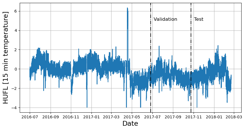
# We are going to plot the temperature of the transformer
# and marking the validation and train splits
u_id = 'HUFL'
x_plot = pd.to_datetime(Y_df[Y_df.unique_id==u_id].ds)
y_plot = Y_df[Y_df.unique_id==u_id].y.values
x_val = x_plot[n_time - val_size - test_size]
x_test = x_plot[n_time - test_size]
fig = plt.figure(figsize=(10, 5))
fig.tight_layout()
plt.plot(x_plot, y_plot)
plt.xlabel('Date', fontsize=17)
plt.ylabel('HUFL [15 min temperature]', fontsize=17)
plt.axvline(x_val, color='black', linestyle='-.')
plt.axvline(x_test, color='black', linestyle='-.')
plt.text(x_val, 5, ' Validation', fontsize=12)
plt.text(x_test, 5, ' Test', fontsize=12)
plt.grid()
```
## 1. Installing NeuralForecast
```python theme={null}
%%capture
!pip install neuralforecast datasetsforecast utilsforecast
```
## 2. Load ETTm2 Data
The `LongHorizon` class will automatically download the complete ETTm2
dataset and process it.
It return three Dataframes: `Y_df` contains the values for the target
variables, `X_df` contains exogenous calendar features and `S_df`
contains static features for each time-series (none for ETTm2). For this
example we will only use `Y_df`.
If you want to use your own data just replace `Y_df`. Be sure to use a
long format and have a similar structure to our data set.
```python theme={null}
import pandas as pd
from datasetsforecast.long_horizon import LongHorizon
# Change this to your own data to try the model
Y_df, _, _ = LongHorizon.load(directory='./', group='ETTm2')
Y_df['ds'] = pd.to_datetime(Y_df['ds'])
# For this excercise we are going to take 20% of the DataSet
n_time = len(Y_df.ds.unique())
val_size = int(.2 * n_time)
test_size = int(.2 * n_time)
Y_df.groupby('unique_id').head(2)
```
| | unique\_id | ds | y |
| ------ | ---------- | ------------------- | --------- |
| 0 | HUFL | 2016-07-01 00:00:00 | -0.041413 |
| 1 | HUFL | 2016-07-01 00:15:00 | -0.185467 |
| 57600 | HULL | 2016-07-01 00:00:00 | 0.040104 |
| 57601 | HULL | 2016-07-01 00:15:00 | -0.214450 |
| 115200 | LUFL | 2016-07-01 00:00:00 | 0.695804 |
| 115201 | LUFL | 2016-07-01 00:15:00 | 0.434685 |
| 172800 | LULL | 2016-07-01 00:00:00 | 0.434430 |
| 172801 | LULL | 2016-07-01 00:15:00 | 0.428168 |
| 230400 | MUFL | 2016-07-01 00:00:00 | -0.599211 |
| 230401 | MUFL | 2016-07-01 00:15:00 | -0.658068 |
| 288000 | MULL | 2016-07-01 00:00:00 | -0.393536 |
| 288001 | MULL | 2016-07-01 00:15:00 | -0.659338 |
| 345600 | OT | 2016-07-01 00:00:00 | 1.018032 |
| 345601 | OT | 2016-07-01 00:15:00 | 0.980124 |
```python theme={null}
import matplotlib.pyplot as plt
# We are going to plot the temperature of the transformer
# and marking the validation and train splits
u_id = 'HUFL'
x_plot = pd.to_datetime(Y_df[Y_df.unique_id==u_id].ds)
y_plot = Y_df[Y_df.unique_id==u_id].y.values
x_val = x_plot[n_time - val_size - test_size]
x_test = x_plot[n_time - test_size]
fig = plt.figure(figsize=(10, 5))
fig.tight_layout()
plt.plot(x_plot, y_plot)
plt.xlabel('Date', fontsize=17)
plt.ylabel('HUFL [15 min temperature]', fontsize=17)
plt.axvline(x_val, color='black', linestyle='-.')
plt.axvline(x_test, color='black', linestyle='-.')
plt.text(x_val, 5, ' Validation', fontsize=12)
plt.text(x_test, 5, ' Test', fontsize=12)
plt.grid()
```
 ## 3. Hyperparameter selection and forecasting
The `AutoNHITS` class will automatically perform hyperparamter tunning
using [Tune library](https://docs.ray.io/en/latest/tune/index.html),
exploring a user-defined or default search space. Models are selected
based on the error on a validation set and the best model is then stored
and used during inference.
The `AutoNHITS.default_config` attribute contains a suggested
hyperparameter space. Here, we specify a different search space
following the paper’s hyperparameters. Notice that *1000 Stochastic
Gradient Steps* are enough to achieve SoTA performance. Feel free to
play around with this space.
```python theme={null}
from ray import tune
from neuralforecast.auto import AutoNHITS
from neuralforecast.core import NeuralForecast
```
```python theme={null}
horizon = 96 # 24hrs = 4 * 15 min.
# Use your own config or AutoNHITS.default_config
nhits_config = {
"learning_rate": tune.choice([1e-3]), # Initial Learning rate
"max_steps": tune.choice([1000]), # Number of SGD steps
"input_size": tune.choice([5 * horizon]), # input_size = multiplier * horizon
"batch_size": tune.choice([7]), # Number of series in windows
"windows_batch_size": tune.choice([256]), # Number of windows in batch
"n_pool_kernel_size": tune.choice([[2, 2, 2], [16, 8, 1]]), # MaxPool's Kernelsize
"n_freq_downsample": tune.choice([[168, 24, 1], [24, 12, 1], [1, 1, 1]]), # Interpolation expressivity ratios
"activation": tune.choice(['ReLU']), # Type of non-linear activation
"n_blocks": tune.choice([[1, 1, 1]]), # Blocks per each 3 stacks
"mlp_units": tune.choice([[[512, 512], [512, 512], [512, 512]]]), # 2 512-Layers per block for each stack
"interpolation_mode": tune.choice(['linear']), # Type of multi-step interpolation
"val_check_steps": tune.choice([100]), # Compute validation every 100 epochs
"random_seed": tune.randint(1, 10),
}
```
> **Tip**
>
> Refer to [https://docs.ray.io/en/latest/tune/index.html](https://docs.ray.io/en/latest/tune/index.html) for more
> information on the different space options, such as lists and
> continous intervals.m
To instantiate `AutoNHITS` you need to define:
* `h`: forecasting horizon
* `loss`: training loss. Use the `DistributionLoss` to produce
probabilistic forecasts.
* `config`: hyperparameter search space. If `None`, the `AutoNHITS`
class will use a pre-defined suggested hyperparameter space.
* `num_samples`: number of configurations explored.
```python theme={null}
models = [AutoNHITS(h=horizon,
config=nhits_config,
num_samples=5)]
```
Fit the model by instantiating a `NeuralForecast` object with the
following required parameters:
* `models`: a list of models.
* `freq`: a string indicating the frequency of the data. (See [panda’s
available
frequencies](https://pandas.pydata.org/pandas-docs/stable/user_guide/timeseries.html#offset-aliases).)
The `cross_validation` method allows you to simulate multiple historic
forecasts, greatly simplifying pipelines by replacing for loops with
`fit` and `predict` methods.
With time series data, cross validation is done by defining a sliding
window across the historical data and predicting the period following
it. This form of cross validation allows us to arrive at a better
estimation of our model’s predictive abilities across a wider range of
temporal instances while also keeping the data in the training set
contiguous as is required by our models.
The `cross_validation` method will use the validation set for
hyperparameter selection, and will then produce the forecasts for the
test set.
```python theme={null}
%%capture
nf = NeuralForecast(
models=models,
freq='15min')
Y_hat_df = nf.cross_validation(df=Y_df, val_size=val_size,
test_size=test_size, n_windows=None)
```
## 4. Evaluate Results
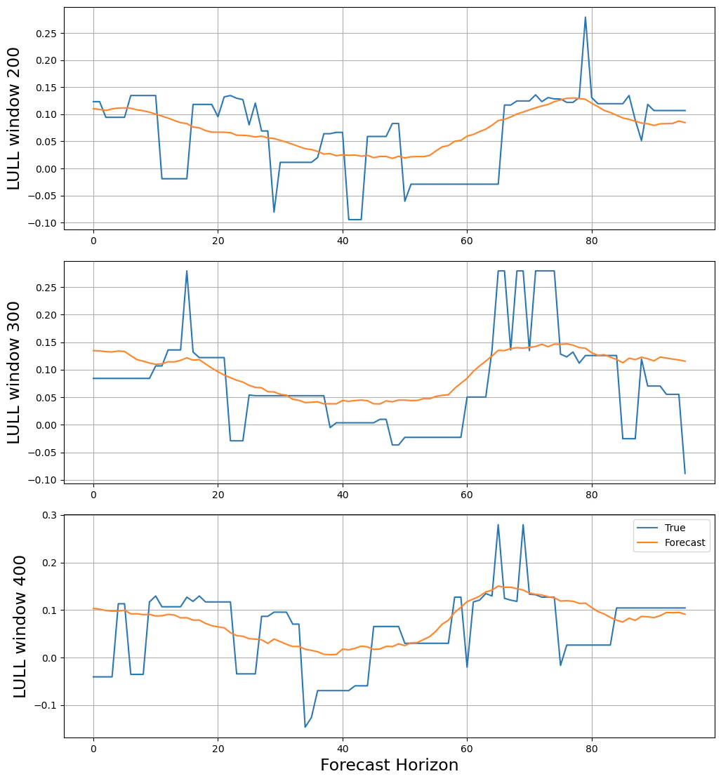
The `AutoNHITS` class contains a `results` tune attribute that stores
information of each configuration explored. It contains the validation
loss and best validation hyperparameter.
```python theme={null}
nf.models[0].results.get_best_result().config
```
```text theme={null}
{'learning_rate': 0.001,
'max_steps': 1000,
'input_size': 480,
'batch_size': 7,
'windows_batch_size': 256,
'n_pool_kernel_size': [2, 2, 2],
'n_freq_downsample': [24, 12, 1],
'activation': 'ReLU',
'n_blocks': [1, 1, 1],
'mlp_units': [[512, 512], [512, 512], [512, 512]],
'interpolation_mode': 'linear',
'val_check_steps': 100,
'random_seed': 8,
'h': 96,
'loss': MAE(),
'valid_loss': MAE()}
```
```python theme={null}
from utilsforecast.plotting import plot_series
series = ['HUFL','HULL','LUFL','LULL','MUFL','MULL','OT']
series_id = series[3] # 'LULL'
series_cutoffs = Y_hat_df.loc[Y_hat_df['unique_id'] == "LULL", 'cutoff'].unique()
for w_idx in [200, 300, 400]:
cutoff = series_cutoffs[w_idx]
plot_df = Y_hat_df.loc[Y_hat_df['cutoff'] == cutoff, ['unique_id', 'ds', 'y', 'AutoNHITS']]
fig = plot_series(
df=plot_df[['unique_id', 'ds', 'y']],
forecasts_df=plot_df[['unique_id', 'ds', 'AutoNHITS']],
ids=[series_id],
models=['AutoNHITS'],
max_insample_length=96
)
display(fig)
```
## 3. Hyperparameter selection and forecasting
The `AutoNHITS` class will automatically perform hyperparamter tunning
using [Tune library](https://docs.ray.io/en/latest/tune/index.html),
exploring a user-defined or default search space. Models are selected
based on the error on a validation set and the best model is then stored
and used during inference.
The `AutoNHITS.default_config` attribute contains a suggested
hyperparameter space. Here, we specify a different search space
following the paper’s hyperparameters. Notice that *1000 Stochastic
Gradient Steps* are enough to achieve SoTA performance. Feel free to
play around with this space.
```python theme={null}
from ray import tune
from neuralforecast.auto import AutoNHITS
from neuralforecast.core import NeuralForecast
```
```python theme={null}
horizon = 96 # 24hrs = 4 * 15 min.
# Use your own config or AutoNHITS.default_config
nhits_config = {
"learning_rate": tune.choice([1e-3]), # Initial Learning rate
"max_steps": tune.choice([1000]), # Number of SGD steps
"input_size": tune.choice([5 * horizon]), # input_size = multiplier * horizon
"batch_size": tune.choice([7]), # Number of series in windows
"windows_batch_size": tune.choice([256]), # Number of windows in batch
"n_pool_kernel_size": tune.choice([[2, 2, 2], [16, 8, 1]]), # MaxPool's Kernelsize
"n_freq_downsample": tune.choice([[168, 24, 1], [24, 12, 1], [1, 1, 1]]), # Interpolation expressivity ratios
"activation": tune.choice(['ReLU']), # Type of non-linear activation
"n_blocks": tune.choice([[1, 1, 1]]), # Blocks per each 3 stacks
"mlp_units": tune.choice([[[512, 512], [512, 512], [512, 512]]]), # 2 512-Layers per block for each stack
"interpolation_mode": tune.choice(['linear']), # Type of multi-step interpolation
"val_check_steps": tune.choice([100]), # Compute validation every 100 epochs
"random_seed": tune.randint(1, 10),
}
```
> **Tip**
>
> Refer to [https://docs.ray.io/en/latest/tune/index.html](https://docs.ray.io/en/latest/tune/index.html) for more
> information on the different space options, such as lists and
> continous intervals.m
To instantiate `AutoNHITS` you need to define:
* `h`: forecasting horizon
* `loss`: training loss. Use the `DistributionLoss` to produce
probabilistic forecasts.
* `config`: hyperparameter search space. If `None`, the `AutoNHITS`
class will use a pre-defined suggested hyperparameter space.
* `num_samples`: number of configurations explored.
```python theme={null}
models = [AutoNHITS(h=horizon,
config=nhits_config,
num_samples=5)]
```
Fit the model by instantiating a `NeuralForecast` object with the
following required parameters:
* `models`: a list of models.
* `freq`: a string indicating the frequency of the data. (See [panda’s
available
frequencies](https://pandas.pydata.org/pandas-docs/stable/user_guide/timeseries.html#offset-aliases).)
The `cross_validation` method allows you to simulate multiple historic
forecasts, greatly simplifying pipelines by replacing for loops with
`fit` and `predict` methods.
With time series data, cross validation is done by defining a sliding
window across the historical data and predicting the period following
it. This form of cross validation allows us to arrive at a better
estimation of our model’s predictive abilities across a wider range of
temporal instances while also keeping the data in the training set
contiguous as is required by our models.
The `cross_validation` method will use the validation set for
hyperparameter selection, and will then produce the forecasts for the
test set.
```python theme={null}
%%capture
nf = NeuralForecast(
models=models,
freq='15min')
Y_hat_df = nf.cross_validation(df=Y_df, val_size=val_size,
test_size=test_size, n_windows=None)
```
## 4. Evaluate Results
The `AutoNHITS` class contains a `results` tune attribute that stores
information of each configuration explored. It contains the validation
loss and best validation hyperparameter.
```python theme={null}
nf.models[0].results.get_best_result().config
```
```text theme={null}
{'learning_rate': 0.001,
'max_steps': 1000,
'input_size': 480,
'batch_size': 7,
'windows_batch_size': 256,
'n_pool_kernel_size': [2, 2, 2],
'n_freq_downsample': [24, 12, 1],
'activation': 'ReLU',
'n_blocks': [1, 1, 1],
'mlp_units': [[512, 512], [512, 512], [512, 512]],
'interpolation_mode': 'linear',
'val_check_steps': 100,
'random_seed': 8,
'h': 96,
'loss': MAE(),
'valid_loss': MAE()}
```
```python theme={null}
from utilsforecast.plotting import plot_series
series = ['HUFL','HULL','LUFL','LULL','MUFL','MULL','OT']
series_id = series[3] # 'LULL'
series_cutoffs = Y_hat_df.loc[Y_hat_df['unique_id'] == "LULL", 'cutoff'].unique()
for w_idx in [200, 300, 400]:
cutoff = series_cutoffs[w_idx]
plot_df = Y_hat_df.loc[Y_hat_df['cutoff'] == cutoff, ['unique_id', 'ds', 'y', 'AutoNHITS']]
fig = plot_series(
df=plot_df[['unique_id', 'ds', 'y']],
forecasts_df=plot_df[['unique_id', 'ds', 'AutoNHITS']],
ids=[series_id],
models=['AutoNHITS'],
max_insample_length=96
)
display(fig)
```
 Finally, we compute the test errors for the two metrics of interest:
$\qquad MAE = \frac{1}{Windows * Horizon} \sum_{\tau} |y_{\tau} - \hat{y}_{\tau}| \qquad$
and
$\qquad MSE = \frac{1}{Windows * Horizon} \sum_{\tau} (y_{\tau} - \hat{y}_{\tau})^{2} \qquad$
```python theme={null}
from utilsforecast.evaluation import evaluate
from utilsforecast.losses import mae, mse
eval_df = evaluate(
df=Y_hat_df.drop(columns=["cutoff"]),
metrics=[mae, mse],
agg_fn="mean"
)
print('MAE: ', eval_df.iloc[0]["AutoNHITS"])
print('MSE: ', eval_df.iloc[1]["AutoNHITS"])
```
```text theme={null}
MAE: 0.24862242128243706
MSE: 0.17257850996828134
```
For reference we can check the performance when compared to previous
‘state-of-the-art’ long-horizon Transformer-based forecasting methods
from the [NHITS paper](https://arxiv.org/abs/2201.12886). To recover or
improve the paper results try setting `hyperopt_max_evals=30` in
[Hyperparameter Tuning](#cell-4).
Mean Absolute Error (MAE):
| Horizon | NHITS | AutoFormer | InFormer | ARIMA |
| ------- | --------- | ---------- | -------- | ----- |
| 96 | **0.249** | 0.339 | 0.453 | 0.301 |
| 192 | 0.305 | 0.340 | 0.563 | 0.345 |
| 336 | 0.346 | 0.372 | 0.887 | 0.386 |
| 720 | 0.426 | 0.419 | 1.388 | 0.445 |
Mean Squared Error (MSE):
| Horizon | NHITS | AutoFormer | InFormer | ARIMA |
| ------- | --------- | ---------- | -------- | ----- |
| 96 | **0.173** | 0.255 | 0.365 | 0.225 |
| 192 | 0.245 | 0.281 | 0.533 | 0.298 |
| 336 | 0.295 | 0.339 | 1.363 | 0.370 |
| 720 | 0.401 | 0.422 | 3.379 | 0.478 |
## References
[Cristian Challu, Kin G. Olivares, Boris N. Oreshkin, Federico Garza,
Max Mergenthaler-Canseco, Artur Dubrawski (2021). NHITS: Neural
Hierarchical Interpolation for Time Series Forecasting. Accepted at AAAI
2023.](https://arxiv.org/abs/2201.12886)
Finally, we compute the test errors for the two metrics of interest:
$\qquad MAE = \frac{1}{Windows * Horizon} \sum_{\tau} |y_{\tau} - \hat{y}_{\tau}| \qquad$
and
$\qquad MSE = \frac{1}{Windows * Horizon} \sum_{\tau} (y_{\tau} - \hat{y}_{\tau})^{2} \qquad$
```python theme={null}
from utilsforecast.evaluation import evaluate
from utilsforecast.losses import mae, mse
eval_df = evaluate(
df=Y_hat_df.drop(columns=["cutoff"]),
metrics=[mae, mse],
agg_fn="mean"
)
print('MAE: ', eval_df.iloc[0]["AutoNHITS"])
print('MSE: ', eval_df.iloc[1]["AutoNHITS"])
```
```text theme={null}
MAE: 0.24862242128243706
MSE: 0.17257850996828134
```
For reference we can check the performance when compared to previous
‘state-of-the-art’ long-horizon Transformer-based forecasting methods
from the [NHITS paper](https://arxiv.org/abs/2201.12886). To recover or
improve the paper results try setting `hyperopt_max_evals=30` in
[Hyperparameter Tuning](#cell-4).
Mean Absolute Error (MAE):
| Horizon | NHITS | AutoFormer | InFormer | ARIMA |
| ------- | --------- | ---------- | -------- | ----- |
| 96 | **0.249** | 0.339 | 0.453 | 0.301 |
| 192 | 0.305 | 0.340 | 0.563 | 0.345 |
| 336 | 0.346 | 0.372 | 0.887 | 0.386 |
| 720 | 0.426 | 0.419 | 1.388 | 0.445 |
Mean Squared Error (MSE):
| Horizon | NHITS | AutoFormer | InFormer | ARIMA |
| ------- | --------- | ---------- | -------- | ----- |
| 96 | **0.173** | 0.255 | 0.365 | 0.225 |
| 192 | 0.245 | 0.281 | 0.533 | 0.298 |
| 336 | 0.295 | 0.339 | 1.363 | 0.370 |
| 720 | 0.401 | 0.422 | 3.379 | 0.478 |
## References
[Cristian Challu, Kin G. Olivares, Boris N. Oreshkin, Federico Garza,
Max Mergenthaler-Canseco, Artur Dubrawski (2021). NHITS: Neural
Hierarchical Interpolation for Time Series Forecasting. Accepted at AAAI
2023.](https://arxiv.org/abs/2201.12886)