> ## Documentation Index
> Fetch the complete documentation index at: https://nixtlaverse.nixtla.io/llms.txt
> Use this file to discover all available pages before exploring further.
# Interpretable Decompositions
[Time series signal
decomposition](https://en.wikipedia.org/wiki/Decomposition_of_time_series)
involves breaking down an original time series into its constituent
components. By decomposing the time series, we can gain insights into
underlying patterns, trends-cycles, and seasonal effects, enabling
improved understanding and forecasting accuracy.
This notebook will show how to use the `NHITS`/`NBEATSx` to extract
these series’ components. We will:
- Installing
NeuralForecast.
- Simulate a Harmonic Signal.
- NHITS’ forecast
decomposition.
- NBEATSx’ forecast decomposition.
You can run these experiments using GPU with Google Colab.
 ## 1. Installing NeuralForecast
```python theme={null}
%%capture
!pip install neuralforecast
```
## 2. Simulate a Harmonic Signal
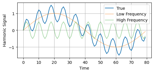
In this example, we will consider a Harmonic signal comprising two
frequencies: one low-frequency and one high-frequency.
```python theme={null}
import numpy as np
import pandas as pd
```
```python theme={null}
N = 10_000
T = 1.0 / 800.0 # sample spacing
x = np.linspace(0.0, N*T, N, endpoint=False)
y1 = np.sin(10.0 * 2.0*np.pi*x)
y2 = 0.5 * np.sin(100 * 2.0*np.pi*x)
y = y1 + y2
```
```python theme={null}
import matplotlib.pyplot as plt
plt.rcParams["axes.grid"]=True
```
```python theme={null}
fig, ax = plt.subplots(figsize=(6, 2.5))
plt.plot(y[-80:], label='True')
plt.plot(y1[-80:], label='Low Frequency', alpha=0.4)
plt.plot(y2[-80:], label='High Frequency', alpha=0.4)
plt.ylabel('Harmonic Signal')
plt.xlabel('Time')
plt.legend()
plt.show()
plt.close()
```
## 1. Installing NeuralForecast
```python theme={null}
%%capture
!pip install neuralforecast
```
## 2. Simulate a Harmonic Signal
In this example, we will consider a Harmonic signal comprising two
frequencies: one low-frequency and one high-frequency.
```python theme={null}
import numpy as np
import pandas as pd
```
```python theme={null}
N = 10_000
T = 1.0 / 800.0 # sample spacing
x = np.linspace(0.0, N*T, N, endpoint=False)
y1 = np.sin(10.0 * 2.0*np.pi*x)
y2 = 0.5 * np.sin(100 * 2.0*np.pi*x)
y = y1 + y2
```
```python theme={null}
import matplotlib.pyplot as plt
plt.rcParams["axes.grid"]=True
```
```python theme={null}
fig, ax = plt.subplots(figsize=(6, 2.5))
plt.plot(y[-80:], label='True')
plt.plot(y1[-80:], label='Low Frequency', alpha=0.4)
plt.plot(y2[-80:], label='High Frequency', alpha=0.4)
plt.ylabel('Harmonic Signal')
plt.xlabel('Time')
plt.legend()
plt.show()
plt.close()
```
 ```python theme={null}
# Split dataset into train/test
# Last horizon observations for test
horizon = 96
Y_df = pd.DataFrame(dict(unique_id=1, ds=np.arange(len(x)), y=y))
Y_train_df = Y_df.groupby('unique_id').head(len(Y_df)-horizon)
Y_test_df = Y_df.groupby('unique_id').tail(horizon)
Y_test_df
```
| | unique\_id | ds | y |
| ---- | ---------- | ---- | --------- |
| 9904 | 1 | 9904 | -0.951057 |
| 9905 | 1 | 9905 | -0.570326 |
| 9906 | 1 | 9906 | -0.391007 |
| 9907 | 1 | 9907 | -0.499087 |
| 9908 | 1 | 9908 | -0.809017 |
| ... | ... | ... | ... |
| 9995 | 1 | 9995 | -0.029130 |
| 9996 | 1 | 9996 | -0.309017 |
| 9997 | 1 | 9997 | -0.586999 |
| 9998 | 1 | 9998 | -0.656434 |
| 9999 | 1 | 9999 | -0.432012 |
## 3. NHITS decomposition
We will employ `NHITS` stack-specialization to recover the latent
harmonic functions.
`NHITS`, a Wavelet-inspired algorithm, allows for breaking down a time
series into various scales or resolutions, aiding in the identification
of localized patterns or features. The expressivity ratios for each
layer enable control over the model’s stack specialization.
```python theme={null}
from neuralforecast.models import NHITS, NBEATSx
from neuralforecast import NeuralForecast
from neuralforecast.losses.pytorch import HuberLoss, MQLoss
```
```python theme={null}
%%capture
models = [NHITS(h=horizon, # Forecast horizon
input_size=2 * horizon, # Length of input sequence
loss=HuberLoss(), # Robust Huber Loss
max_steps=1000, # Number of steps to train
dropout_prob_theta=0.5,
interpolation_mode='linear',
stack_types=['identity']*2,
n_blocks=[1, 1],
mlp_units=[[64, 64],[64, 64]],
n_freq_downsample=[10, 1], # Inverse expressivity ratios for NHITS' stacks specialization
val_check_steps=10, # Frequency of validation signal (affects early stopping)
)
]
nf = NeuralForecast(models=models, freq=1)
nf.fit(df=Y_train_df)
```
```python theme={null}
from neuralforecast.tsdataset import TimeSeriesDataset
# NHITS decomposition plot
model = nf.models[0]
dataset, *_ = TimeSeriesDataset.from_df(df = Y_train_df)
y_hat = model.decompose(dataset=dataset)
```
```text theme={null}
GPU available: True (cuda), used: True
TPU available: False, using: 0 TPU cores
HPU available: False, using: 0 HPUs
LOCAL_RANK: 0 - CUDA_VISIBLE_DEVICES: [0]
```
```text theme={null}
Predicting: | | 0/? [00:00
## 4. NBEATSx decomposition
Here we will employ `NBEATSx` interpretable basis projection to recover
the latent harmonic functions.
`NBEATSx`, this network in its interpretable variant sequentially
projects the signal into polynomials and harmonic basis to learn trend
$T$ and seasonality $S$ components:
$\hat{y}_{[t+1:t+H]} = \theta_{1} T + \theta_{2} S$
In contrast to `NHITS`’ wavelet-like projections the basis heavily
determine the behavior of the projections. And the Fourier projections
are not capable of being immediately decomposed into individual
frequencies.
```python theme={null}
%%capture
models = [NBEATSx(h=horizon, # Forecast horizon
input_size=2 * horizon, # Length of input sequence
loss=HuberLoss(), # Robust Huber Loss
max_steps=1000, # Number of steps to train
dropout_prob_theta=0.5,
stack_types=['trend', 'seasonality'], # Harmonic/Trend projection basis
n_polynomials=0, # Lower frequencies can be captured by polynomials
n_blocks=[1, 1],
mlp_units=[[64, 64],[64, 64]],
val_check_steps=10, # Frequency of validation signal (affects early stopping)
)
]
nf = NeuralForecast(models=models, freq=1)
nf.fit(df=Y_train_df)
```
```python theme={null}
# NBEATSx decomposition plot
model = nf.models[0]
dataset, *_ = TimeSeriesDataset.from_df(df = Y_train_df)
y_hat = model.decompose(dataset=dataset)
```
```text theme={null}
GPU available: True (cuda), used: True
TPU available: False, using: 0 TPU cores
HPU available: False, using: 0 HPUs
LOCAL_RANK: 0 - CUDA_VISIBLE_DEVICES: [0]
```
```text theme={null}
Predicting: | | 0/? [00:00
## References
* [Cristian Challu, Kin G. Olivares, Boris N. Oreshkin, Federico
Garza, Max Mergenthaler-Canseco, Artur Dubrawski (2023). NHITS:
Neural Hierarchical Interpolation for Time Series
Forecasting.](https://arxiv.org/abs/2201.12886)
```python theme={null}
# Split dataset into train/test
# Last horizon observations for test
horizon = 96
Y_df = pd.DataFrame(dict(unique_id=1, ds=np.arange(len(x)), y=y))
Y_train_df = Y_df.groupby('unique_id').head(len(Y_df)-horizon)
Y_test_df = Y_df.groupby('unique_id').tail(horizon)
Y_test_df
```
| | unique\_id | ds | y |
| ---- | ---------- | ---- | --------- |
| 9904 | 1 | 9904 | -0.951057 |
| 9905 | 1 | 9905 | -0.570326 |
| 9906 | 1 | 9906 | -0.391007 |
| 9907 | 1 | 9907 | -0.499087 |
| 9908 | 1 | 9908 | -0.809017 |
| ... | ... | ... | ... |
| 9995 | 1 | 9995 | -0.029130 |
| 9996 | 1 | 9996 | -0.309017 |
| 9997 | 1 | 9997 | -0.586999 |
| 9998 | 1 | 9998 | -0.656434 |
| 9999 | 1 | 9999 | -0.432012 |
## 3. NHITS decomposition
We will employ `NHITS` stack-specialization to recover the latent
harmonic functions.
`NHITS`, a Wavelet-inspired algorithm, allows for breaking down a time
series into various scales or resolutions, aiding in the identification
of localized patterns or features. The expressivity ratios for each
layer enable control over the model’s stack specialization.
```python theme={null}
from neuralforecast.models import NHITS, NBEATSx
from neuralforecast import NeuralForecast
from neuralforecast.losses.pytorch import HuberLoss, MQLoss
```
```python theme={null}
%%capture
models = [NHITS(h=horizon, # Forecast horizon
input_size=2 * horizon, # Length of input sequence
loss=HuberLoss(), # Robust Huber Loss
max_steps=1000, # Number of steps to train
dropout_prob_theta=0.5,
interpolation_mode='linear',
stack_types=['identity']*2,
n_blocks=[1, 1],
mlp_units=[[64, 64],[64, 64]],
n_freq_downsample=[10, 1], # Inverse expressivity ratios for NHITS' stacks specialization
val_check_steps=10, # Frequency of validation signal (affects early stopping)
)
]
nf = NeuralForecast(models=models, freq=1)
nf.fit(df=Y_train_df)
```
```python theme={null}
from neuralforecast.tsdataset import TimeSeriesDataset
# NHITS decomposition plot
model = nf.models[0]
dataset, *_ = TimeSeriesDataset.from_df(df = Y_train_df)
y_hat = model.decompose(dataset=dataset)
```
```text theme={null}
GPU available: True (cuda), used: True
TPU available: False, using: 0 TPU cores
HPU available: False, using: 0 HPUs
LOCAL_RANK: 0 - CUDA_VISIBLE_DEVICES: [0]
```
```text theme={null}
Predicting: | | 0/? [00:00
## 4. NBEATSx decomposition
Here we will employ `NBEATSx` interpretable basis projection to recover
the latent harmonic functions.
`NBEATSx`, this network in its interpretable variant sequentially
projects the signal into polynomials and harmonic basis to learn trend
$T$ and seasonality $S$ components:
$\hat{y}_{[t+1:t+H]} = \theta_{1} T + \theta_{2} S$
In contrast to `NHITS`’ wavelet-like projections the basis heavily
determine the behavior of the projections. And the Fourier projections
are not capable of being immediately decomposed into individual
frequencies.
```python theme={null}
%%capture
models = [NBEATSx(h=horizon, # Forecast horizon
input_size=2 * horizon, # Length of input sequence
loss=HuberLoss(), # Robust Huber Loss
max_steps=1000, # Number of steps to train
dropout_prob_theta=0.5,
stack_types=['trend', 'seasonality'], # Harmonic/Trend projection basis
n_polynomials=0, # Lower frequencies can be captured by polynomials
n_blocks=[1, 1],
mlp_units=[[64, 64],[64, 64]],
val_check_steps=10, # Frequency of validation signal (affects early stopping)
)
]
nf = NeuralForecast(models=models, freq=1)
nf.fit(df=Y_train_df)
```
```python theme={null}
# NBEATSx decomposition plot
model = nf.models[0]
dataset, *_ = TimeSeriesDataset.from_df(df = Y_train_df)
y_hat = model.decompose(dataset=dataset)
```
```text theme={null}
GPU available: True (cuda), used: True
TPU available: False, using: 0 TPU cores
HPU available: False, using: 0 HPUs
LOCAL_RANK: 0 - CUDA_VISIBLE_DEVICES: [0]
```
```text theme={null}
Predicting: | | 0/? [00:00
## References
* [Cristian Challu, Kin G. Olivares, Boris N. Oreshkin, Federico
Garza, Max Mergenthaler-Canseco, Artur Dubrawski (2023). NHITS:
Neural Hierarchical Interpolation for Time Series
Forecasting.](https://arxiv.org/abs/2201.12886)
* [Boris N. Oreshkin, Dmitri Carpov, Nicolas Chapados, Yoshua Bengio
(2019). “N-BEATS: Neural basis expansion analysis for interpretable
time series forecasting”.](https://arxiv.org/abs/1905.10437)
* [Kin G. Olivares, Cristian Challu, Grzegorz Marcjasz, Rafał Weron,
Artur Dubrawski (2021). “Neural basis expansion analysis with
exogenous variables: Forecasting electricity prices with
NBEATSx”.](https://arxiv.org/abs/2104.05522)